Written by Sig Silber
This week we focus on oil and gas. We are not addressing the short-term fluctuations in oil and gas prices related to the weather. That is a legitimate topic but one that is best handled if we published on that topic daily as weather reports change fast. Instead we are focused on the War on Fossil Fuels that is related to Global Warming. That is a lot more interesting to me and I assume is of interest to more people. We also have a discussion of one aspect of farm economics in the article. We cover the drought and of course, we provide our Intermediate-Term Weather forecast. We always include a lot of other information in this report including tonight the status of the major reservoirs in California.

Please share this article – Go to the very top of the page, right-hand side, for social media buttons. Please feel free to send this article to anyone who you think might benefit from reading it.
First let’s discuss oil and gas. I will begin by presenting some information from a report done for the State of Wyoming. You can find the full report here. It covers Wyoming and a number of other Western States. You will see what states are covered in subsequent exhibits. It does not include Texas.
First we start with a little history and some forecasts which presumably were the EIA reference case at the time this report was prepared. A new EIA report came out on February 3, 2021 and we will discuss that also.

This is a pretty busy graphic showing historical production and price of two commodities and a forecast. It takes into account the impact of COVID-19 and presumably the EIA reference forecast makes assumptions about the recovery of the use of oil and gas but makes no assumptions about changes in government policy. It is sort of a Business as Usual (BAU) Reference Scenario and is a starting point for analysis. I present it because the subsequent exhibits are based on the assumptions shown here. This includes
One of the assumptions is that after 2031, oil development in the Arctic Wildlife Refuge (ANWR) is expected to occur. I probably would not have included that in the reference case. But this Wyoming Report is more narrow in scope but addressed two potential actions the New Administration in Washington might take, one of which they have promised to take.

I am not trying to argue ideology here. But this graphics shows the steep decline curve of oil production if no more wells are drilled. Just imagine that the Gray and Orange/Yellow is removed. I will say that there are some assumptions made here namely that if drilling on Federal Land is prohibited (the orange/yellow is removed) why assume that there is not more drilling on private and state owned land?

This is the same as above but this one is for Natural Gas. Again the assumption that drilling is prohibited on Federal Land directly results in less NG is not a good assumption. It is a good assumption for Wyoming as essentially all their drilling is on Federal Land. And Wyoming funded the preparation of this report.

Again to be clear I am not taking sides on this issue but using analysis prepared for one purpose to shed light on the impact of oil and gas. So here you see what the investment would be for the gray and yellow/orange slices on the chart. If the industry makes the investiments this shows the size of the investment. If they are precluded this shows the investment that does not happen. Two scenarios are shown here. One is existing permits on Federal Land can be drilled but no more permits issued and the other is no drilling on Federal Land. Again it may be more of a problem for some companies than others but there is also state owned land and private land. So I am certainly not endorsing the analysis but when you are writing an article, you have to use the information that is available. And of course this is a Western States analysis not an analysis for the entire U.S. This is mostly important with respect to natural gas which is produced in large quantities in the East. .
Investment is payments to employees and contractors and things that are purchased.

Obviously, there are price assumptions in the study used to convert physical units into dollars. One might look at this as very related to the impact on the import export budget of the U.S.

This shows the tax revenue lost. It is broken down by state.

Supposedly this is the value added lost to the economy. “These impacts are estimated in this study by using economic multipliers from the Bureau of Economic Analysis (BEA) in the US Department of Commerce. These so-called Type I multipliers include the direct and the indirect impacts from oil and gas spending on the supply chain supporting oil and gas drilling and extraction.” Thus the esitimates in this table does not include induced impacts based on the purchases made by employees.
It is not my intention to critique the report but I will say that the multiplier effects, if they exist, probably are spread over many different states. I have only reviewed the summary of the report and I think it provides a good starting point for understanding the importance of oil and gas
One might ask “what does this have to do with weather”? Weather impacts the demand for energy. Weather might impact the supply of energy. And weather to the extent that it is associated with Climate Change impacts government actions that might reduce the amount of activity in the oil and gas sector.

And this summarizes the above.
And now let us take a look at the EIA (Energy Information Agency) new forecast. I am presenting it (Their Annual Energy Outlook AEO which can be found here) even though I consider it to be mostly a pile of rubbish but it is information that is used. I guess it depends on how you use their report. I should not complain that they have a lot of subordinate slides that show how they get to the summary slides but that works better for the reader than for someone like myself who is trying to capture the meat within the forecast and I keep finding tiny bones when I look at the full report. So I am sorry that I come across as being critical when it really is simply frustration that I am finding it difficult to to write this article tonight.
Here goes:
I had planned to start with some slides used in their summary presentation and then add some more from the report. But I could not find anything in the full report worth reporting. So I am just presenting the summary.

This is the introductory slide in their Press Release version of the report

This is a short-term view of how we might come out of the Pandemic and it seems reasonable to me

This is a transition slide and presumably they will address the three bullet points above in the next three parts of the presentation

So this shows the assumptions used to prepare the Reference Case. They do address different scenarios but the scenarios addressed do not include actions to reduce GHG Emissions. But I guess it is a decent way to do an analysis.

So here they show what they did and on the right is where someone might list the changes in policy and probably show the list on the left except the middle row rightmost cell where you deviate from the reference case to the hypothetic or real changes in laws and regulatons. We looked at some of that in the first presentation that preceded this one.

So these are the highlights of the report and for each highlight there are a small number of graphics that relate to that highlight.

Here they have three scenarios for economic growth and the energy use for each scenario. I could have added a slide that shows a decline in energy use per dollar of GDP and perhaps I will try to find that one again but the trend is a decline in energy use per dollar of GDP and depending on the sources of energy this translates into a larger or smaller decline in GHG emissions per dollar of GDP.

On the left are economic sectors. On the right, energy sources.

I left this one out originally based on its score on the Lame Index but decided to add it for comleteness. Remember this is the reference case and what they are showing is simply that the sector where there is growth in their fantasy is industrial (rather than services). It looks like they conclude that the growth of the industrial sector will lead to more consumption of LPG (liquid petroleum gas). The graphic artists used by EIA employees or contractors are not the most skilled at creating graphics that someone can read and comprehend.

This could be a good slide and perhaps it is. But the assumption that future growth will be in the industrial sector rather than services is highly questionable to me.

So here they go into scenarios but the scenarios assume no changes in policy.

Some (e.g. California and General Motors) think that transportation might be using electricity sooner.

I have my own way of showing scenarios but in the U.S. there is freedom to confuse.

Here they look at two scenarios in addition to the Reference Case. One case has more oil and gas than the reference case and one has less.The one with less might be useful if one factored in what seems to be a drag on oil and gas production. Again the graphic artists do not make reading these graphics easy.

Now they look at Imports and Exports. Again remember this is the reference case. It is not clear what would make supply lower or higher.

For production they have four scenarios in addition to the Reference Case. On the right they show the change in exports that would be expected. There is no discussion of what comes first the chicken or the egg. I am not going to critique their report in detail but there may be more scenarios than shown here. High prices tend to lead to supply increases but low prices sometimes lead to demand increases. Given that oil and gas will be competing with solar and wind etc., the cross elasticities would seem to be important and I can not tell if that was taken into account.

If you can figure out the graphic I think it says that the industrial sector grows the most and shrinks the most if there is more or less natural gas. The graphic seems to lump oil and gas together but probably few will notice.

A startling observation that if oil and gas are in increased supply they will be exported and if there is less oil and gas the exports will be less. Can you really get paid to produce this kind of a report?

This marks the end of their summary. I may find some exhibits from the full report which can be found
here. They have a lot of slides But they all relate to the Reference Case. Is there anyone out there that thinks the Reference Case will be what actually happens? But it might be that the approach here is actually a good approach.
Remember this is their Reference Case which assumes no change in level of government intervention and probably some other unrealistic assumptions. It does reflect what the EIA thinks they know about technology trends.
Conclusion
I have presented two ways to look at things and I conclude that it is not easy to predict the future of oil and gas. Both presentations are useful.
They both provide useful information.
They both were developed for different purposes.
If you believe the second presentation, you would probably not invest in wind energy.
If you believe the first presentation, you might want to hope for a moratorium on drilling public land and buy up those leases as such a moratorium might not be able ot be maintained.
So even though I am frustrated with both reports, I do see the value in them.
Severe Weather

There is some snow. But looking ahead to Spring runoff it does not look great but it is looking better than it has recently.

Blue and green are good and orange and red are not. You can see where things look bad and where they look ok for the Spring runoff.

There are a number of California reservoirs that do not look so good.

Here is more information on atmospheric rivers.
Let’s look at the current drought situation.

And the week to week change

There basically was no change in the drought this week.
Here we look at four-time periods: one week, one month, six months, and a full year.

You kind of have to look at this 4-Plex in reverse. The lower right map shows the situation today as compared to a year ago. This set of graphics shows that this drought has materialized over the past year.
It is easy to get confused by this graphic. The map in the lower right does not show that the drought was worse a year ago but the change from a year ago to today. So the drought now is much worse than a year ago.
The result is very dry soil conditions

Fire risk is high in some areas and there are and will be environmental negative impacts.
February Drought Outlook
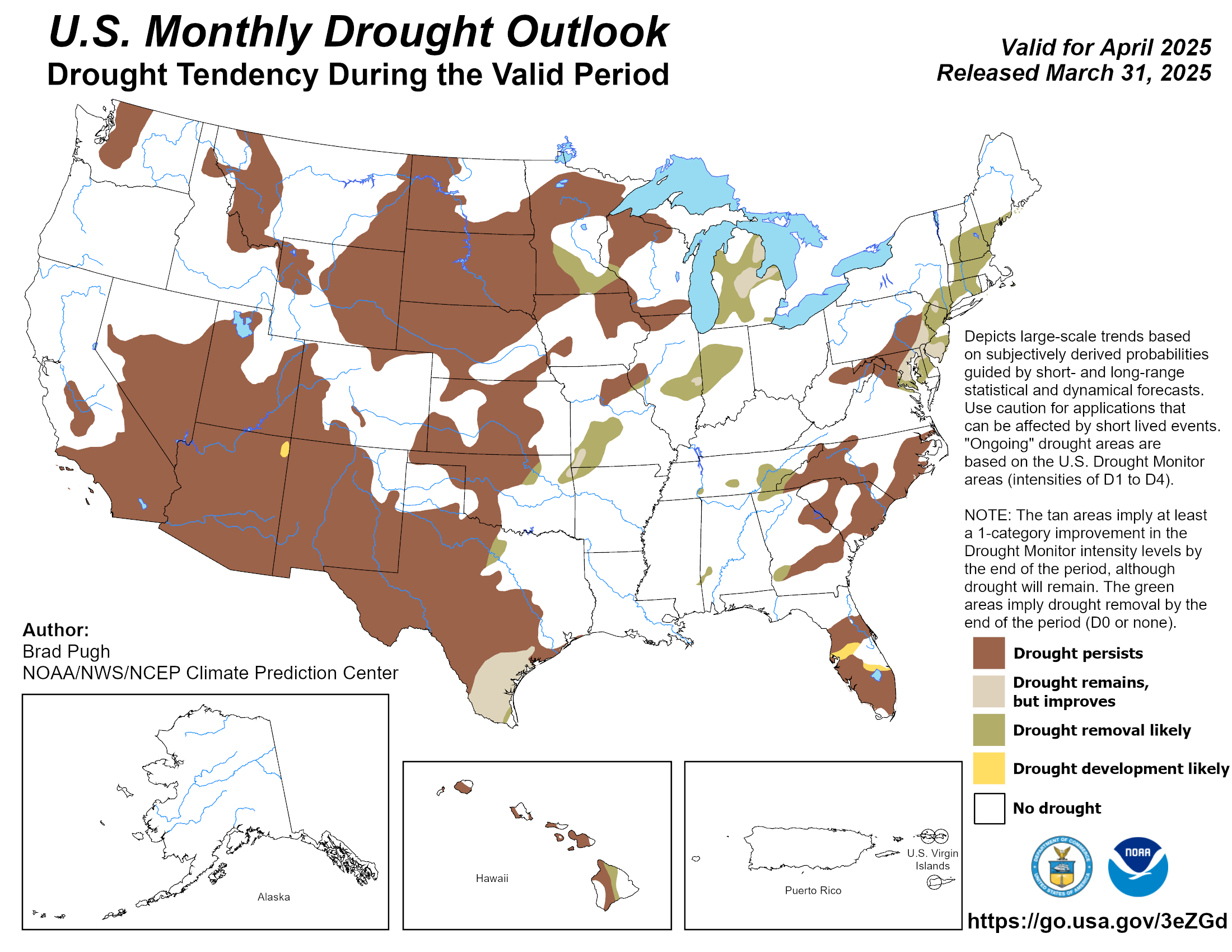
The forecast is for dry. But not all La Nina’s are dry. There is a lot of variation.

That situation has improved a lot.

This situation has improved also.
Intermediate-Term Weather Forecast
Showing from left to right, Days 1- 5, 6 – 10, 8 – 14, and Weeks 3 – 4 You can click on these maps to have them enlarge. Also, the discussions that go with these forecast maps can be found here (first two weeks) and here (Weeks 3 and 4).
First Temperature
And then Precipitation
A short burst of winter perhaps. But it soon reverts to a typical La Nina situation.
The Week 3-4 Discussion is always interesting.
Week 3-4 Forecast Discussion Valid Sat Feb 20 2021-Fri Mar 05 2021
La Nina conditions currently are present across the Pacific Ocean. Equatorial sea surface temperatures (SSTs) are below average from the west-central to eastern Pacific Ocean with enhanced trade winds and westerly wind anomalies aloft. The RMM-based Madden-Julian Oscillation (MJO) index indicates a considerable increase in amplitude of the intraseasonal signal over the western Pacific. Both the ECMWF and GEFS continue to favor the eastward propagation of intraseasonal signal across the western Pacific during week-1, with increased spread in the ensemble means among the models during week-2. The Week 3-4 temperature and precipitation outlooks are based primarily on dynamical model forecasts from the NCEP CFS, ECMWF, and JMA, and the Subseasonal Experiment (SubX) multi-model ensemble (MME) of experimental and operational ensemble prediction systems with additional considerations for La Nina and long-term trends, as well as the predicted evolution of the pattern from Week-2 forecasts.
Good agreement exists among the dynamical models regarding the anomalous 500-hPa height pattern over the week 3-4 period. Dynamical model 500hPa height anomaly forecasts during week 3-4 show a fairly consistent evolution from the forecast state during Week-2. The NCEP CFS, ECMWF and JMA Models feature anomalous ridging with above normal 500-hPa heights over the North Pacific and southwestern Alaska extending eastward into most of the southern CONUS, consistent with a La Nina, while anomalous troughing with below normal 500-hPa heights are forecast over the northwestern CONUS and eastern Mainland Alaska. All models appear consistent in predicting near to above normal 500-hPa heights over Hawaii.
Above normal temperatures are expected across much of the southern tier of the CONUS under predicted above normal 500-hPa heights and the eastward flow of warm Pacific air, in a circulation pattern that is consistent with La Nina. Near to below normal 500-hPa heights lead to enhanced probabilities of below normal temperatures across much of the northeastern CONUS except for Maine, where above normal temperatures are indicated, consistent with the Autoblend and Manual tools. Anomalous northerly flow results in increased probabilities of below normal temperatures for southern Mainland Alaska and the Alaska Panhandle as well as the Aleutians, while decadal trends lead to predicted above normal temperatures for northern Mainland Alaska.
The dynamical model guidance is in reasonably good agreement on the spatial pattern of anomalous precipitation during the Week 3-4 period. Below normal precipitation is favored throughout most of the southern tier of the US, consistently predicted in dynamical and statistical guidance. Anomalous troughing and several shortwave disturbances lead to enhanced probabilities of above normal precipitation over parts of the Northern Rockies and the Northern High Plains. Anomalous northerly flow leads to increased probabilities of below normal precipitation for most of central and southern Mainland Alaska, the Alaska Panhandle, and the Aleutians, while above normal precipitation is likely over northwestern Mainland Alaska, supported by the CFS/ECMWF/JMA Equal Weighted tools as well as the Autoblend and Manual tools.
SST anomalies around Hawaii remain above normal, leading to an increased probability of above normal temperatures throughout the forecast period. The SubX MME anomaly forecast and the GEFSv12 probabilities indicate likely above median precipitation for the week 3-4 period for Hawaii.
Farm Profitability
This is only one part of the picture but we have some information so I am presenting it. I am only presenting the summary but the full report can be found here.

Off hand that does not look so good when prices received are down and prices paid are up

Comparing December 2020 to December 2019 it looks like prices received increased a bit but prices paid increased more. But there were other payments made to farmers and I do not think those payments are included here. Like many things, One has to really dig to figure out what any of this reporting means. I provided a link to the full and long report so that is probably more useful depending on what part of agriculture one is involved in.
Cattle Report

It looks like there has been a slight decline in the cattle inventory. The full report can be found
here.
International

This week we do not have a map.
Good everywhere except the U.S.
In the box are shown the major resources we use. We will not be using them all each week but the reader is welcome to refer to these resources.
Major Sources of Information Used in this Weekly Report - The U.S. Drought Monitor (the full report can be accessed here)
- Selected graphics from our other Weather and Climate Reports are repeated in this report. These reports can be accessed by referencing the Directory here
- Selections from the Tuesday USD Weather and Crop Bulletin (the full report can be accessed here). Selections from the USDA Office of the Chief Economist can be found here. NASS Executive Briefings can be found here. A wide range of NASS Reports can be found here. USDA Foreign Agriculture Service Briefs can be found here and here. Other useful sources of information that I regularly utilize are the National Integrated Drought Information System (NIDIS) which can be accessed here and the USDA NRCS Weekly and Weather Climate Update which can be accessed here. A glossary of terms can be found here.
|
.