Written by Sig Silber
In the near term, it looks like hot weather will be around in populated areas from Boston to Baltimore due to a high pressure system parked over the area. Historically that sort of weather can precipitate riots and kids opening water hydrants which can interfere with firefighting. I have made my first attempt at comparing the current El Nino with the Monster El Nino of 1997/1998. My analysis at this point is a work in progress but I am sharing what I have come up with and expect to expand the analysis for the August 17 Weather and Climate Report. All comments are welcome. Summer continues and there are signs that the Monsoon may become reinvigorated but impacting a smaller number of states above Arizona and New Mexico than usual. Forecasters are having a hard time pinning it down possibly due to a complex weather pattern that I will discuss in this report.

This is the Regular Edition of my weekly Weather and Climate Update Report. Additional information can be found here on Page II of the Global Economic Intersection Weather and Climate Report. Additional information can be found here on Page II of the Global Economic Intersection Weather and Climate Report.
Let us discuss perhaps the most famous El Nino ever (although the 1982/1983 El Nino is famous also). I have been able to include the links to the NOAA graphics in the following NOAA Discussion (so you can click on the Figures indicated in the article) but not the links that move you between sections of the article as GEI does not support those commands and they complicate reading the article. You can read the article in the original by going to the El Nino of 1997/1998 . The purpose of this discussion is to compare and contrast the current El Nino with the World Champion 1997/1998 El Nino. The text in the report is the complete article from NOAA. I have selectively added some of their graphics into the article here so you do not have to click on those to see them. Also, I have added some graphics from the current El Nino for comparison and some of my comments as [Editor’s Notes].
As mentioned above, my analysis is still a work in progress. I may do some additional work on it during the week and present a more complete analysis in my August 17 Weather and Climate Report or at a later time. Let’s face it. Every El Nino is different so it is not easy to compare one to another. But the comparison may be informative and helpful to those who can benefit from additional insight into how this El Nino may evolve. And it is important to remember that for CONUS, the major impacts are likely during Fall so the data I am presenting is prior to the full impact of this El Nino, not a retrospective. Not everyone will want to wade through this detailed and highly technical analysis so they can scroll down to the section on current weather conditions and forecasts. .
From what I see so far, It suggests that this El Nino is not going to match the 1997/1998 El Nino but it is closer to it than one might think. I suspect the Faux El Nino of 2014/2015 discharged some of the energy in the ENSO battery or we might be having a record matching or beating El Nino right now. Also, and not much discussed, this El Nino is arriving early and thus may have lesser impacts on the Northern Hemisphere. One thing I have learned from attempting this comparison is that El Nino is very much about the Southern Hemisphere and not much information is presented on that in the NOAA Weekly ENSO Update.
From the CPC.NCEP.NOAA Report on this subject, with the link provided above, Very strong 1997-98 Pacific warm episode (El Niño)
1. Overview
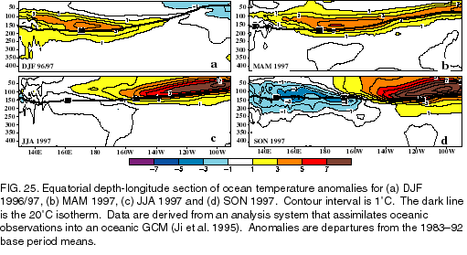
The global climate during 1997 was affected by one of the strongest Pacific warm episodes on record. These warm episode conditions developed rapidly in March, with strong ENSO conditions persisting from May through the end of the year (and subsequently well into 1998) (Figs. 20, 21 ). During this episode the abnormally warm SSTs which covered the eastern half of the equatorial Pacific (Fig. 21a) were comparable in magnitude and areal extent to the famed 1982/83 El Niño (Fig. 20a). These 1997 warm episode conditions were accompanied by a strong negative phase of the Southern Oscillation, with the equatorial Southern Oscillation Index (SOI) also comparable in magnitude to that observed during 1982/83 (Fig. 20b). Also evident since April was a markedly reduced strength of the low-level (850-hPa) equatorial easterly winds across the eastern tropical Pacific (Fig. 21c). At times these anomalies indicated a complete disappearance of the easterlies across the entire eastern Pacific, along with a complete collapse of the normal equatorial Walker circulation. These anomalies were also comparable to those observed during the 1982/83 El Niño (Fig. 20c).
The above conditions were associated with a dramatic alteration of the global pattern of tropical rainfall and deep tropical convection, as indicated by above-normal rainfall across the eastern half of the tropical Pacific and by significantly below-normal convection across Indonesia and the western equatorial Pacific (Fig. 22). The combined zonal extent of these rainfall anomalies covered a distance more than one-half the circumference of the earth.
Selected impacts associated with these warm episode conditions included 1) excessive rainfall across the eastern half of the tropical Pacific, 2) significantly below-normal rainfall and drought across Indonesia and the western tropical Pacific, 3) below-normal hurricane activity over the North Atlantic during August-October, with a simultaneously expanded region of conditions favorable for tropical cyclone formation over the eastern subtropical North Pacific 4) excessive rainfall and flooding in equatorial eastern Africa during October-December 5) a dramatic eastward extension of the South Pacific jet stream to well east of the date line during June-December which resulted in enhanced storminess across southeastern South America and central Chile and abnormally dry conditions across the Amazon Basin, central America, the Caribbean Sea and the subtropical North Atlantic throughout the period.
2. Evolution of the 1997 El Nino
The year began with a continuation of weak cold episode conditions in the tropical Pacific during December 1996-February 1997 (DJF 1996/97). These conditions included a well-defined tongue of abnormally cold SSTs extending across the eastern tropical Pacific (Fig. 23b), with equatorial SSTs greater than 28°C confined to the area west of the date line (Fig. 23a). SSTs were slightly below normal in the Niño 1+2 region (Fig. 24a), the Niño 3 region (Fig. 24b) and the Niño 3.4 region (Fig. 24c), and substantially below the 28°C threshold for convection (Gadgil et al. 1984) in all three regions
[Editors Note: I have added a graphic which has two sets of information. The left-hand figure is the long-run history of the Nino 3.4 reading which in the U.S. is the major way of tracking the phases of ENSO i.e. El Nino versus Neutral versus La Nina. It goes back to 1950 so you can easily see the 1997/1998 El Nino there followed by a long La Nina and then a series of weak El Nino’s. It is easy to follow that graphic and you can see how rapid the buildup was in the Nino 3.4 reading which is often referred to as the ONI the Ocean Nino Index. On the right is more recent information but not just for the ONI which is the second row down but for four Nino Indices representing different areas along the Tropical Pacific and they go from west to east with the Nino 1 + 2 being a little south of the Equator to cover Equador and Peru. You can see that it has not been as dramatic a rise although one always has to be careful when reading a graph to be aware of the way the X and Y axis are structured. There was the Faux El Nino in the winter of 2014/2015 which was a false start and probably drained some of the energy from this warm event which otherwise would probably be even stronger and rival the 1997/1998 El Nino. You can see that until recently it has been mostly a Central Pacific warm event (Nino 4) which some call a Modoki. We clearly are in an El Nino now but the Nino 1+2 area SST anomalies appear to have peaked and leveled off. There is a lot of information in this combined graphic. It does not auto-update but NOAA updates this information weekly in their ENSO Report so it is avaiable.]

The colder-than-normal conditions were accompanied by a strongly sloping equatorial oceanic thermocline (Fig. 25a), with increased thermocline depths across the western Pacific and reduced depths over the extreme eastern Pacific [The center of the thermocline is approximated by the 20°C isotherm]. These variations in thermocline depth were accompanied by abnormally warm ocean temperatures in the western and central tropical Pacific between 50-200 m depth and by abnormally cold water in the eastern tropical Pacific between the surface and 50-100 m depth. During this period, the atmosphere featured 1) a positive phase of the Southern Oscillation, with below-normal sea level pressure (SLP) across the western tropical Pacific (Fig. 21b), 2) a broad area of slightly enhanced low-level easterlies across the central tropical Pacific (Figs. 21c, 26a ), 3) enhanced tropical convection over Indonesia and the western tropical Pacific [indicated by negative values of anomalous Outgoing Longwave Radiation (OLR)] and suppressed convection in the vicinity of the date line (Fig. 26a), and 4) westerly wind anomalies at upper levels across the eastern tropical Pacific (Fig. 27a). Collectively, these conditions reflected an enhanced equatorial Walker circulation and a continued coupling between the positive phase of the Southern Oscillation and below-normal SSTs across the eastern tropical Pacific.
In contrast, March and April featured an extremely rapid transition to one of the strongest warm episodes of the century. SSTs increased nearly 1.5°C over the normal annual cycle in the Niño 1+2 region during March (Fig. 24a), and nearly 1.0°-1.5°C over the annual cycle in the Niño 3, Niño 3.4 and Niño 4 regions. In the Niño 4 region this increase occurred during a two-week period and was greater than the entire annual cycle of SST for that region. A second period of very rapid SST increases in the east-central Pacific then occurred during April, as SSTs in both the Niño 3 and Niño 3.4 regions climbed an additional 1°C over that expected from the normal annual cycle. Thus, by mid-April SSTs exceeded 28°C across the central and east-central equatorial Pacific (Figs. 24b-d ), with values averaging 1°-3°C above normal in all four Niño regions. Area-averaged SSTs in the Niño 3, Niño 3.4 and Niño 4 regions then remained nearly constant at values greater than 28°C throughout the remainder of the year. This warming reflected a nearly complete elimination of the annual cycle in SSTs across most of the equatorial Pacific, which is normally characterized by a peak in temperatures during March-April and a minimum during September-October.
For the MAM season as a whole, mean SSTs greater than 29°C extended to east of the date line, and values greater than 28°C extended to approximately 160°W (Fig. 23c). These temperatures averaged 0.5°-2.0°C above normal across the central and east-central tropical Pacific (Fig. 23d). This warming was accompanied by increased depths of the oceanic thermocline everywhere east of the date line (Fig. 25b), and by a flattening of the thermocline across the region. In the eastern tropical Pacific, this suppressed thermocline reflected substantially reduced oceanic upwelling in association with a weakening of the low-level equatorial easterly winds (westerly wind anomalies) (Fig. 26b ). These conditions were accompanied by suppressed convection throughout Indonesia and enhanced convection in the vicinity of the date line, which is opposite to the pattern observed the previous season.
Editor’s Note: Although labeled Outgoing Longwave Radiation Anomalies the OLR (description from NOAA: Negative (Positive) OLR are indicative of enhanced (suppressed) convection and hence more (less) cloud coverage typical of El Niño (La Niña) episodes. More (Less) convective activity in the central and eastern equatorial Pacific implies higher (lower), colder (warmer) cloud tops, which emit much less (more) infrared radiation into space) is a surrogate for precipitation with blue being wet and the red shades being dry. So in MAM we had the suppressed convection in the Western Pacific and increased precipitation near the Date Line. But we have not yet had the 1997/1998 shift in precipitation to the Eastern Pacific. In fact there has not been much chance since May. You can also look back on this Hovmoeller and see the Faux El Nino of 2014/2015 and see why I never concluded that it was real].
During JJA, SSTs remained very warm throughout the entire eastern half of the tropical Pacific, with the 29°C isotherm expanding eastward to approximately 150°W, and the 28°C isotherm extending eastward to approximately 125°W (Fig. 23e ). These extremely warm waters are highly abnormal for that time of year (Fig. 23f), a period normally characterized by a marked decrease in SSTs across the eastern tropical Pacific. As a result, SST anomalies increased substantially throughout the region, and exceeded 3°- 4°C between 130°W and the west coast of South America (Fig. 23f). [Editor’s Note we are currently running about 2.6C and I do not think it will increase but it might. So this El Nino is just under the 1997/1998 El Nino on that metric.]. This increase in anomalies was accompanied by a further flattening of the oceanic thermocline across the eastern Pacific (Fig. 25c), as the 20°C isotherm dropped to more than 100 m depth and ocean temperatures increased to more than 7°C above normal between 50-125 m depth. [Editor’s Note: It this case it has been 6C but mostly 5C. However one has to keep in mind the base keeps on being adjusted by NOAA due to a trend that may be Global Warming or may be the PDO but the main point is that anomalies and absolute values are not the same thing. So the subsurface water temperature is slightly higher than the anomaly indicates.]
[Editor’s Note: I incorporated Figure 25 from the NOAA report directly in the discussion because of its importance so you do not need to call up that link.]
[Editor’s note: for comparison purposes this is the current subsurface Thermocline situation
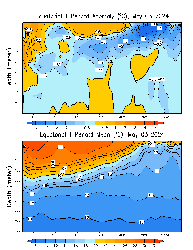
[Editor’s Note: One of the things I notice is that our current conditions correspond to the Sep-Oct-Nov conditions in 1997 with just a slight difference in intensity.
It is difficult to read the NOAA graphic for 1997 but it looks like an anomaly of 7C and the most extreme we have had is 6C over a smaller area of the subsurface. At this time of the year in 1997 the warm anomaly covered a much larger extent of the Equator. There was no sign of an Upwelling Wave to signal the end of the Kelvin Wave Activity. I have sensed that we have been in the final stages of this El Nino and this analysis makes me more confident that what I have sensed is indeed correct. At one point it seemed that his was an El Nino that arrived late but that was because we were considering the Faux El Nino of 2014 as a warm event that was slow in getting started. Now I am thinking what we have is a warm event that is peaking early. I am also thinking that the weather services may not be sufficiently taking that into account in their long-term forecasts]
The JJA period also featured an increasingly negative phase of the Southern Oscillation, and a further decrease in the strength of the 850-hPa easterly winds (3-6 m s-1 below normal) across most of the central and eastern tropical Pacific (Fig. 26c ). These conditions were accompanied by increased tropical convection (Fig. 26c) and rainfall across the entire eastern half of the Pacific, and by decreased rainfall across the western tropical Pacific and Indonesia. These changes in tropical convection reflected 1) a pronounced eastward extension of the primary area of tropical convection to well east of the date line, and at times an actual shift of the main region of tropical convection to the eastern half of the tropical Pacific (not shown), and 2) a strengthening and equatorward shift of the intertropical convergence zone (ITCZ) in the Northern Hemisphere (not shown). [Editor’s Note: I thought I would show what things look like this year compared with the very powerful 1996-1997-1998 El Nino. Notice the SOI went very negative early in 1997. Also notice it went positive the following Spring.

And here is the current reporting of the SOI

The 1997 El Nino came on suddenly. This one has had a gradual build up re the increasingly negative SOI ] Also observed during JJA was the development of an anomalous upper-level anticyclonic circulation in the Southern Hemisphere subtropics between the date line and 90°W (Fig. 27c). This feature is a recurring aspect of the winter hemisphere circulation during strong warm episodes (Arkin 1982), and reflects several important changes in the flow occurring in the Tropics, the subtropics and the extratropics. In the Tropics, the equatorward flank of the circulation anomaly reflects anomalous upper-level easterly flow across the eastern Pacific, and thus comprises important structural elements of the much weaker-than-normal equatorial Walker circulation observed during the period. In the subtropics, above-normal heights (not shown) accompanying the anticyclonic circulation anomaly reflect an eastward extension of the mean subtropical ridge to well east of the date line, in response to the increase in tropical convection and deep tropospheric heating across the eastern tropical Pacific. In the extratropics, the anomalous anticyclonic circulation is an integral component of the coupling process between changes in tropical convection and changes in the wintertime jet stream across the South Pacific. The Southern Hemisphere circulation was also characterized by recurring high-latitude blocking over the high latitudes of the eastern South Pacific, a feature typical of strong warm episode conditions (Karoly, 1989).Strong warm episode conditions continued during SON (Figs. 23g, h), with SSTs greater than 28°C extending eastward from Indonesia to 125°W and greater than 29°C extending eastward to approximately 140°W (Fig. 23g). The normal cold-tongue that typically occupies the eastern half of the tropical Pacific at this time of the year was notably absent, consistent with the collapse of the normal annual cycle in SSTs throughout the region (Figs. 24b, c). A nearly isothermal temperature structure was also observed from the surface to 150 m depth, with ocean temperatures exceeding 9°C above normal at 50-150 m depth in the eastern Pacific (Fig. 25d).
Also during SON, El Niño-related enhanced rainfall and heavy tropical convection developed across equatorial eastern Africa. This rainfall was associated with low-level easterly wind anomalies across the tropical Indian Ocean (Fig. 26d), and with a continuation of extremely suppressed convection throughout Indonesia. Also observed was a continuation of enhanced upper-level westerlies and an extended jet stream across the subtropical South Pacific (Fig. 27d), resulting in continued heavy precipitation across Chile and southeastern South America. Elsewhere, above-normal rainfall and increased storminess developed across the Gulf Coast of the United States (Fig. 22), in association with enhanced upper-level westerlies across the southern tier of the country.
3. Equatorial Walker Circulation
Over the equatorial Pacific the divergent component of the atmospheric circulation is intimately related to the distribution of tropical convection, which in turn is an integral part of the still larger Southern Oscillation (Bjerknes 1969). This divergent circulation is often partitioned into its zonal and meridional components, respectively called the equatorial Walker circulation and the tropical Hadley circulation. The equatorial Walker circulation is characterized by ascending motion over Indonesia and the western tropical Pacific, and descending motion over the east-central equatorial Pacific, with upper-level westerly (low-level easterly) flow completing the “direct” circulation cell. Following Halpert and Bell (1997), we illustrate the equatorial Walker circulation using pressure-longitude plots of the vector field whose horizontal component is the divergent zonal wind and whose vertical component is the scaled pressure vertical velocity. The pressure vertical velocity was subjectively scaled to give a sense of the relative vertical motion in the equatorial plane. The seasonal mean equatorial Walker circulation and anomalies during 1997, along with the accompanying seasonal relative humidity anomalies, are shown in Fig. 28.
During DJF 1996/97, a well-defined equatorial Walker circulation was present (Fig. 28a), with ascending motion over the western tropical Pacific, descending motion over the eastern Pacific and a circulation center near 170°W. These conditions reflected a slight strengthening and an overall westward shift of the circulation center compared to normal (Fig. 28b), consistent with weak cold episode conditions and a positive phase of the Southern Oscillation. These conditions dissipated rapidly during MAM 1997, as a near-normal strength and location of the Walker circulation prevailed (Figs. 28c, d).
By JJA 1997, ascending motion and deep tropical convection encompassed the tropical Pacific between 140°E and 120°W (Fig. 28e ), while no well-defined pattern of vertical motion was evident over Indonesia. This anomalous vertical motion field (Fig. 28f) reflected a nearly complete disappearance of the equatorial Walker circulation. The pattern was also accompanied by enhanced relative humidity everywhere east of the date line, and by reduced relative humidity across the western tropical Pacific and Indonesia. These conditions strengthened during SON 1997, with the equatorial Walker circulation again nearly absent (Figs. 28g, h).
4. South Pacific jet stream during July-September 1997
In both the Northern and Southern Hemisphere, the extratropical wintertime jet stream over the western and central Pacific is intimately related to the distribution of tropical convection across Indonesia and the tropical Pacific. Thus, the interannual variability of these jet streams is strongly influenced by the ENSO. During strong El Niño conditions the wintertime jet stream extends eastward to well east of the date line, and over the eastern Pacific is shifted well equatorward from normal. These changes in the jet stream reflect a deep baroclinic jet structure often extending across the entire Pacific Basin, along with a pronounced eastward shift of the normal jet exit region to well east of the date line. These conditions then contribute to enhanced storminess and above-normal precipitation at lower latitudes of both North and South America.
During 1997, the South Pacific jet stream was particularly impacted during July-September by the ongoing strong El Niño conditions, while the primary impacts on the North Pacific jet stream did not occur until early 1998. Thus, this analysis focuses on the wintertime South Pacific jet stream, which extended across the entire South Pacific and brought enhanced storminess and above-normal precipitation throughout Chile and southeastern South America [Editor’s Note” This longer current animation shows how the Jet Stream is crossing the Pacific. Perhaps the followin graphic which includes a discussion of how the Polar Jet Stream is usually impacted by ENZO will be helpful]

[Editors’s Note: I have not seen this happening. In general the Jet Stream has been further north rather than further south. This may change in the coming months.]
The core of the South Pacific jet stream (approximated by wind speeds greater than 50 m s-1) during July-September is typically located between 22.5°-32.5°S and extends eastward from eastern Australia to approximately 150°W (Fig. 29a ). The jet entrance region is normally located over eastern Australia, and is characterized by a local maximum in along-stream increases in geostrophic wind speed. Additional characteristics of the entrance region include confluent geostrophic flow at upper levels and a strong poleward component of the horizontal ageostrophic flow directed toward lower geopotential height. This ageostrophic flow is one component of the thermodynamically direct, transverse ageostrophic circulation typical of any midlatitude jet entrance region (Palmen and Newton 1969, sections 1.5 and 8.3; Hoskins et al. 1978, Keyser and Shapiro 1986), and produces the required westerly momentum and kinetic energy increases that air parcels experience as they approach the jet core.
Farther downstream, the jet exit region is normally found between the date line and approximately 125°W, and is characterized by a local maximum in along-stream decreases in geostrophic wind speed. Characteristic features of this exit region include diffluent geostrophic flow at upper levels and a strong equatorward component of the ageostrophic flow directed toward higher geopotential height. This ageostrophic flow is one component of the required thermodynamically indirect, transverse ageostrophic circulation typical of any midlatitude jet exit region, and produces the required westerly momentum and kinetic energy decreases that air parcels experience as they exit the jet.
The July-September 1997 period featured an eastward extension of the jet stream across the entire South Pacific (Fig. 29b), and an extension of the jet core to 105°W (nearly 45° east of normal). This extension was accompanied by a pronounced eastward shift in the regions of along-stream decreases in geostrophic wind speed and strong diffluent geostrophic flow, and by a nearly complete elimination of these features in the vicinity of the climatological mean jet exit region. Collectively, these conditions reflected an eastward shift in the location of the jet exit region to between 130°-90°W. This dramatic structural change in the jet stream was accompanied by a dynamically consistent eastward shift in the primary region of equatorward-directed ageostrophic flow at upper levels to the observed jet exit region, indicating a corresponding shift in the entire thermodynamically indirect, transverse ageostrophic circulation that characterizes the jet exit region.
This jet extension and eastward shift of the jet exit region were intimately related to an eastward extension of the subtropical ridge to well east of the date line, which is identified by a well-defined anticyclonic circulation anomaly across the entire eastern subtropical South Pacific during JJA and SON (Figs. 27c, d). Additional aspects of this link between the two features are revealed by examining their common attributes. One common feature is the region of enhanced westerlies over the eastern South Pacific, which comprises both the poleward flank of the anticyclonic circulation anomaly and the extended South Pacific jet stream (compare Figs. 27c, and 29b, c). Two additional common features are the poleward flow and equatorward flow along the western and eastern flanks of the anticyclonic anomaly, respectively, which contain important dynamical information regarding links between the anomalous subtropical ridge and changes in the jet entrance and exit regions.
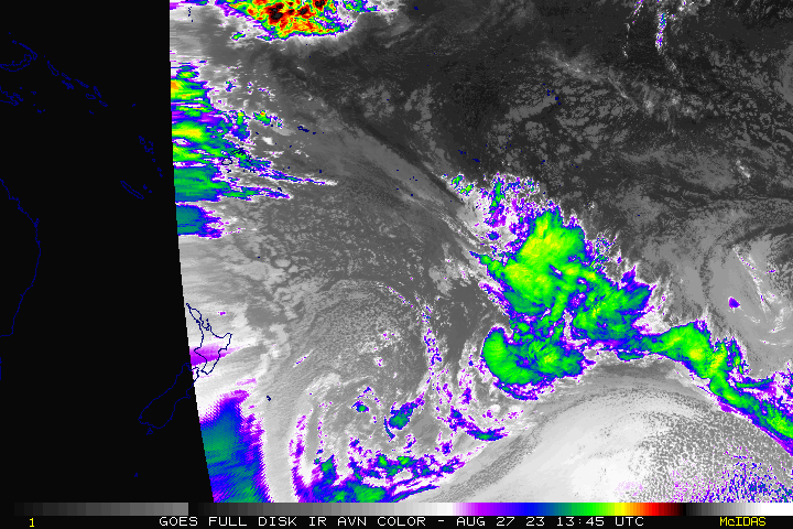
[Editor’s Note: Here is a better look at the current Western Pacific.]
[Editor’s Note: But this is the North Pacific not the South Pacific. Below is the South Pacific but I am not sufficiently familiar with that graphic to fit it into the discussion but it is amusing to see low pressure areas spinning clockwise. But I was expecting to see a giant anti-cyclone and I do not see it. I do see westerlies. I have more work to do!]
The anomalous poleward flow comprises several important structural changes occurring in the exit region of the climatological mean Pacific jet. First, it contributes to anomalous geostrophic confluence throughout the region (Fig. 29c), which also coincides with the entrance region of the anomalous westerly wind maximum. Second, it comprises a dynamically consistent pattern of anomalous ageostrophic flow at upper-levels, directed toward lower geopotential heights at an angle nearly orthogonal to the jet axis. This ageostrophic flow reflects an anomalous thermodynamically direct, transverse ageostrophic circulation, and results in abnormally strong Lagrangian increases in kinetic energy throughout the region (Fig. 30a). In this particular case, both the rotational (Fig. 30b) and divergent (Fig. 30c) components of the ageostrophic flow contributed strongly to these kinetic energy tendencies. Collectively, these anomalies are consistent with an almost complete elimination of the normal jet exit region in the vicinity of the date line, and with a reduced strength of its attendant transverse ageostrophic circulation.
A similar examination indicates that the equatorward flow along the eastern flank of the anticyclonic circulation anomaly comprises important structural and dynamical features of the observed jet exit region. For example, this equatorward flow contributes to geostrophic diffluence in the observed jet exit region (Fig. 30c), an area which also coincides with the exit region of the anomalous westerly wind maximum. The equatorward flow also comprises a coherent pattern of ageostrophic flow directed toward higher geopotential heights at upper levels, at an angle nearly orthogonal to the jet axis. This ageostrophic component of the flow reflects the well-defined thermodynamically indirect, transverse ageostrophic circulation previously noted in the jet exit region, and results in Lagrangian decreases in kinetic energy throughout the area (Fig. 30a). In this case, the rotational component of the ageostrophic flow contributes more to these kinetic energy tendencies (Fig. 30b) than does the divergent component (Fig. 30c).
Thus, in this case the anomalous poleward and equatorward flow found respectively along the western and eastern flanks of the anticyclonic circulation anomaly are strongly linked to jet dynamical processes through El Niño-related changes in the subtropical ridge. These flow features also highlight the jet-like character of the anomalous westerly wind maximum found along the poleward flank of the anticyclonic circulation anomaly.
Switching from the Updated August Outlook to the Current (Right Now to 5 Days Out) Weather Situation:
A more complete version of this report with daily forecasts is available in Part II. This is a summary of that fuller report. This link Worldwide Weather: Current and Three-Month Outlooks: 15 Month Outlooks will take you directly to that set of information but in some Internet Browsers it may just take you to the top of Page II where there is a TABLE OF CONTENTS and you may have to wait for a few seconds for your Browser to redirect to the selected section with that Page or if that process is very slow you can simply lick a second time within the TABLE OF CONTENTS to get to that specific part of the webpage.
First, here is a national 12 hour to 60 hour forecast of weather fronts shown as an animation. Beyond 60 hours, the maps are available at the link provided above.
The explanation for the coding used in these maps, i.e. the full legend, can be found here.
The map below is the mid-atmosphere 7-Day chart rather than the surface highs and lows and weather features. In some cases it provides a clearer less confusing picture as it shows only the major pressure gradients. You can see the location of the Four Corners area where Utah, Colorado, Arizona, and New Mexico meet. At this time of the year there is typically a high pressure system near that area and it is called the Four Corners High. When the Four Corners High is centered directly over the Four Corners area, it creates pretty much a block for the Sonoran Monsoon which only visits its northern neighbor when the highs and lows are located in a way that draws the moist air north. Small changes in the location of that feature make a big difference in the weather of probably about ten or more states. Note the Day 7 location of the Four Corners High is now projected to be near the Four Corners area. This is likely to constrain the Monsoonal activity to Arizona and from there possibly north. But that is not the conclusion that NOAA has presented today. This High moves around a lot so by the time you view this report, it most likely it will be located somewhere else. The models are moving it around run to run and each location results in a different circulation pattern plus the jet stream is involved although I am not showing those graphics here (but they are available on Page II of this Report). If you know where the High is, you can always imagine the clockwise circulation and how that might impact the movement of moisture in from the Gulf of Mexico and up from Mexico and in from the Gulf of California. So this graphic can be very very useful. And it auto-updates, I think every six hours. Even without a weather map, you generally can figure it out. Wind to your back, High to your right, Low to your left.
In the Tropical Weather Outlook graphic below, notice that there is no Pacific Tropical Storm projected to be close enough to the coast to impact CONUS. That is why two weeks ago I raised the question as to a possible temporary break in the action. That is common in the Summer for CONUS. The Sonoran Monsoon which we commandeered and renamed the North American Monsoon or the Southwest Monsoon is a series of bursts and pauses in activity as it impacts the ten or so states in CONUS with the major impacts being with respect to New Mexico and Arizona. That break in the action occurred and after about a week or so the pause ended with the Monsoon regaining its impact on CONUS. But another weak period within the Monsoon occurred this past week and the forecast now is for the Monsoonal Plume to reenter CONUS and tend to be cemtered over the Arizona/New Mexico border. The models change their minds almost daily if not every six hours. I am doing the final editing on this weeks edition of my report in a lightning storm and hope to complete it before power gets knocked out.
.
The below graphic is harder to look at but provides more detail on the water vapor being generated by these storms and the normal summer action of the Southwest Monsoon. It covers a much larger area within CONUS so you can see where the moisture currently is and is going. At this point in time one sees Monsoonal Moisture entering CONUS via Arizona and New Mexico. But notice this water vapor is not moving very far to the north and is currently influencing about five or six states not ten or twelve.

Looking at an even larger area, below is a view which highlights the surface highs and the lows re air pressure on Day 6 (Day 3 can be seen in Part II of this Report). The Eastern Pacific Subtropical High is no longer serving as a total block to all storms attempting to move from the Pacific into CONUS.But it still plays a role in directing most of our weather north into Canada or along the Northern Tier of CONUS and it impacts the positioning of the Four Corners High and thus the strength and location of the Monsoon.
Outlook Days 6 – 14 (but only showing the 8 – 14 Day Maps)
Let’s more ahead to today August 10.
And here is the updated August Temperature Outlook Issued on July 31, 2015.

And here is the current 8 – 14 Day Temperature Outlook which will auto-update and thus be current when you view it. It covers the week following the current week. Today’s 6 – 14 Day Outlook is just nine days of the month and the map shown below of the 8 to 14 day Outlook only shows seven days. The 6 – 10 Day Map is available on Page II of this report. As I view this map on August 10 (it updates each day), it suggests that mid-August may be quite a bit warmer especially for the eastern part of CONUS than originally anticipated.

And here is the Updated Precipitation Outlook for August released on July 31, 2015.

Below is the current 8 – 14 Day Precipitation Outlook which will auto-update daily and thus be current when you view it. And again remember that this map shows only seven days and the 6 – 14 Day map is available on Page II of this report. As I view this map on August 10 (it updates each day), the short-term precipitation outlook is a lot more complicated than the Monthly Outlook for August.

Here are excerpts from the NOAA discussion released today August 10, 2015.
6-10 DAY OUTLOOK FOR AUG 16 – 20 2015
TODAY’S MODELS ARE IN FAIR AGREEMENT ON THE PREDICTED 500-HPA FLOW PATTERN DURING THE 6-10 DAY PERIOD. MOST MODELS DEPICT TROUGHS TO THE WEST OF ALASKA AND WEST OF THE PACIFIC NORTHWEST, AND OVER EASTERN CANADA, AND RIDGING OVER THE EASTERN CONUS AND SOUTHERN ALASKA. THE ECMWF ENSEMBLE HOWEVER INDICATES LITTLE OR NO TROUGHING NEAR THE PACIFIC NORTHWEST AND ABOVE-NORMAL HEIGHTS OVER THE WEST. IN THE OFFICIAL BENDED HEIGHT PATTERN, 500-HPA HEIGHTS ARE PREDICTED TO BE ABOVE-NORMAL OVER WESTERN ALASKA, THE U.S. WEST COAST AND THE NORTHEAST CONUS. 500-HPA HEIGHTS ARE WEAKLY BELOW-NORMAL OVER CENTRAL CANADA INTO PARTS OF THE NORTHERN PLAINS AND OVER THE U.S. SOUTHEAST.
PREDICTED ABOVE-NORMAL HEIGHTS OVER THE WEST COAST AND OVER THE NORTHEAST INCREASES THE CHANCES OF ABOVE-NORMAL TEMPERATURES IN THESE AREAS. SURFACE H IGH-PRESSURE LEADS TO ABOVE-NORMAL TEMPERATURES OVER THE U.S. EAST. RIDGING AND PREDICTED ABOVE-NORMAL HEIGHTS OVER ALASKA ENHANCES THE CHANCES OF ABOVE-NORMAL TEMPERATURES FOR ALASKA. NEAR TO BELOW-NORMAL HEIGHTS OVER THE NORTHERN PLAINS INCREASE THE CHANCES OF BELOW-NORMAL TEMPERATURES IN PARTS OF THE REGION.
ENHANCED MONSOONAL FLOW INCREASES THE LIKELIHOOD OF ABOVE-MEDIAN PRECIPITATION FOR PARTS OF THE SOUTHWEST, NORTHWARD INTO THE NORTHERN PLAINS AND GREAT LAKES REGION. SURFACE FLOW AROUND A REGION OF HIGH PRESSURE OVER THE EAST DRAWS MOISTURE NORTHWARD FROM THE GULF OF MEXICO LEADING TO ENHANCED CHANCES OF ABOVE-MEDIAN PRECIPITATION FOR THE GULF COAST STATES.
FORECAST CONFIDENCE FOR THE 6-10 DAY PERIOD: ABOUT AVERAGE, 3 OUT OF 5, DUE TO FAIR AGREEMENT AMONG THE MODELS AND TOOLS.
8-14 DAY OUTLOOK FOR AUG 18 – 24 2015
ENSEMBLE MODEL FORECASTS FOR THE 8-14 DAY PERIOD INDICATE A SIMILAR HEIGHT PATTERN TO THE 6-10 DAY PERIOD FORECASTS WITH SOME VARIATIONS AND A SLIGHT EASTWARD PROGRESSION. ABOVE-NORMAL HEIGHTS OVER THE NORTHEAST INCREASE IN MAGNITUDE IN THE 8-14 DAY PERIOD, WHILE ABOVE-NORMAL HEIGHTS OVER THE WEST ARE FORECAST TO DECREASE.
THE CONTINUATION OF PREDICTED ABOVE-NORMAL HEIGHTS OVER THE NORTHEAST INCREASES THE CHANCES OF ABOVE-NORMAL TEMPERATURES FOR THE REGION. ABOVE-NORMAL TEMPERATURES CONTINUE TO BE MOST LIKELY FOR THE WEST, WHILE PROBABILITIES HAVE DECREASED. SURFACE HIGH-PRESSURE CONTINUES ABOVE-NORMAL TEMPERATURES OVER THE U.S. EAST. PREDICTED ABOVE-NORMAL HEIGHTS AND TEMPERATURES OVER SOUTHERN ALASKA CONTINUE INTO THE 8-14 DAY PERIOD. BELOW-NORMAL TEMPERATURES ARE MOST LIKELY IN PARTS OF THE NORTHERN PLAINS.
ENHANCED MONSOONAL FLOW INCREASES THE LIKELIHOOD OF ABOVE-MEDIAN PRECIPITATION FOR PARTS OF THE SOUTHWEST, WHILE ABOVE-MEDIAN PRECIPITATION CONTINUES TO BE MOST LIKELY FOR THE WESTERN GREAT LAKES REGION. SURFACE FLOW AROUND A REGION OF HIGH PRESSURE OVER THE EAST CONTINUES TO DRAW MOISTURE NORTHWARD FROM THE GULF OF MEXICO LEADING TO ENHANCED CHANCES OF ABOVE-MEDIAN PRECIPITATION FOR THE GULF COAST STATES.
FORECAST CONFIDENCE FOR THE 8-14 DAY PERIOD IS: BELOW AVERAGE, 2 OUT OF 5, DUE TO FAIR AGREEMENT AMONG THE ENSEMBLE MEANS, INCREASING ENSEMBLE SPREAD, AND SOME DISAGREEMENT AMONG THE TOOLS.
Analogs to Current Conditions
Now let us take a detailed look at the “Analogs” which NOAA provides related to the 5 day period centered on 3 days ago and the 7 day period centered on 4 days ago. “Analog” means that the weather pattern then resembles the recent weather pattern and was used in some way to predict the 6 – 14 day Outlook.
Here are today’s analogs in chronological order although this information is also available with the analog dates listed by the level of correlation. I find the chronological order easier for me to work with. There is a second set of analogs associated with the outlook but I have not been analyzing this second set of information. This first set applies to the 5 and 7 day observed pattern prior to today. The second set which I am not using relates to the forecast outlook 6 – 10 days out to similar patterns that have occurred in the past during the dates covered by the 6 – 10 Day Outlook. That may also be useful information but they put this set of analogs in the discussion with the other set available by a link so I am assuming that this set of analogs is the most meaningful.
Analog Centered Day | ENSO Phase | PDO | AMO | Other Comments |
| 1957 August 5 | El Nino | + | + | Probably a Modoki |
| 1968 August 24 | El Nino | Neutral | – | Modoki Type II |
| 1973 August 23 | La Nina | – | – | |
| 1978 August 15 | Neutral | – | – | |
| 1980 August 18 | Neutral | + | Neutral | |
| 1982 August 12 | El Nino | + | – | Strong late El Nino |
| 1984 August 23 | Neutral | + | – | Just before a La Nina |
The first thing I noticed is that today is August 10 and these are analogs centered on dates 3 or 4 days ago which for six of the non-duplicative analogs are dates in the future. Are we going to experience weather that normally would occur about one or two weeks later in the summer? The 1982 powerful El Nino is interesting..Overall, the analogs are slightly El Nino-ish but other than the 1982 El Nino are not very convincing. Again like last week, the analogs suggest to me that the current El Nino is not going to impact our weather significantly over the next two weeks. The ocean phases associated with the analogs this week are also not very convincing but do suggest that the it is the Atlantic not the Pacific that is in control of our weather. The seminal work on the impact of the PDO and AMO on U.S. climate can be found here.

You may have to squint but the drought probabilities are shown on the map and also indicated by the color coding with shades of red indicating higher than 25% of the years are drought years (25% or less of average precipitation for that area) and shades of blue indicating less than 25% of the years are drought years. Thus drought is defined as the condition that occurs 25% of the time and this ties in nicely with each of the four pairs of two phases of the AMO and PDO.
Historical Anomaly Analysis
When I see the same dates showing up often I find it interesting to consult this list.
Progress of the Warm Event
Let us start with the SOI.
Below is the Southern Oscillation Index (SOI) reported by Queensland, Australia. The first column is the tentative daily reading, the second is the 30 day moving/running average and the third is the 90 day moving/rolling average.
| Date | Current Reading | 30-Day Average | 90 Day Average |
| 4 August 2015 | -39.0 | -14.23 | -14.00 |
| 5 August 2015 | -32.9 | -15.43 | -14.17 |
| 6 August 2015 | -25.9 | -16.74 | -14.10 |
| 7August 2015 | -19.7 | -17.52 | -13.79 |
| 8 August 2015 | -16.0 | -18.16 | -13.48 |
| 9 August 2015 | -4.3 | -18.21 | -13.08 |
| 10 August 2017 | -4.6 | -18.35 | -12.74 |
This past week has continued to be consistent with the continued development of the current El Nino although the SOI values have declined (become less negative) each day this week. The 30-day average, which is the most widely used measure, on August 10 was reported as being -18.35 which is clearly an El Nino reading and due to the high daily values earlier in the week even more extreme than the prior week. The 90-day average also is solidly in El Nino territory at -12.74. The SOI is clearly indicative of an El Nino Event in progress..
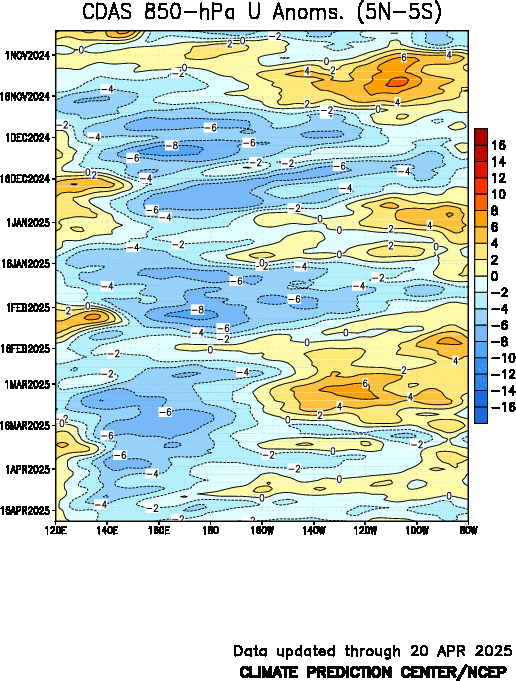
Here are the low-level wind anomalies. This graphic is not as compact as the graphic provided by the weekly NOAA ENSO Report (more white space) but this version auto-updates so you will always have the latest version of this Hovmoeller. There has been another mid-Pacific wind burst in the Date Line to 160W area and yet again from 160E to the Data Line. This is consistent with an active SOI.
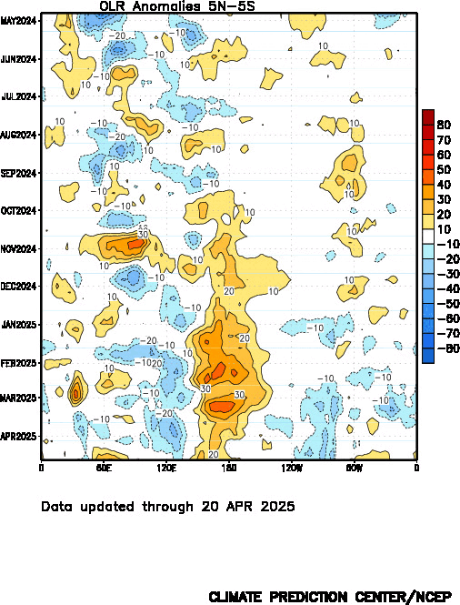
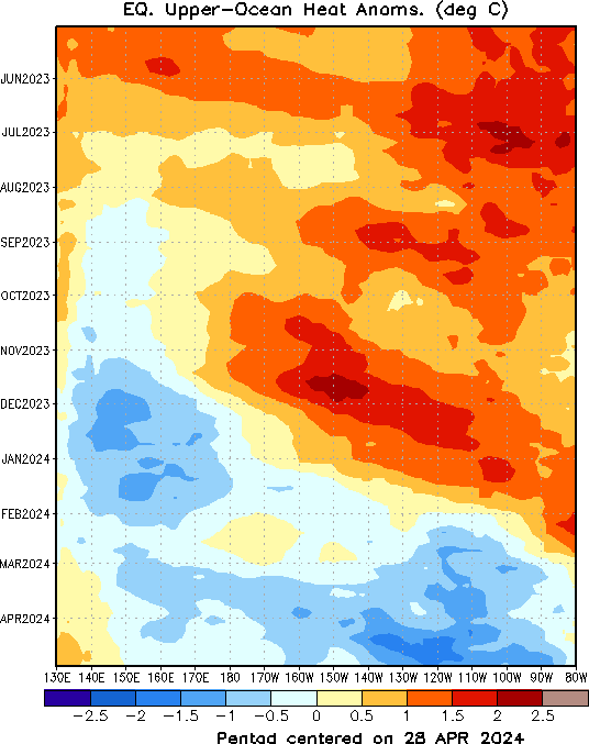
Here is another graphic that is less compact than the prettied up version published by NOAA on Mondays but which has the advantage of auto-updating. You can see how the convection pattern (really cloud tops has since May shifted to the East from a Date Line (180) Modoki pattern to a 170W to 120W Traditional/Canonical El Nino Pattern. But recently the signs of an El Nino are getting quite faint and shifting to the west. The probably impacts on CONUS are thus lessened. The impacts of an El Nino during the summer in the Northern Hemisphere are subtle.
I have discussed this graphic in the earlier analysis of the 1997/1998 El Nino but I am repeating it here to avoid having it be necessary for people to jump around in this report.
Let us now take a look at the progress of the Kevin wave which is the key to the situation. Since February there have been three successive downwelling Kelvin Waves without really an upwelling Kelvin Wave to counter their impact. The first wave which started in February was the most effective at getting this El Nino started. The second wave reinforced to some extent but not much and this third (and I believe last) downwelling Kelvin Wave has created an El Nino that will have a major peak coming soon and possible a second smaller peak.
The main impact of this latest Kelvin Wave has already moved east to 170W where it is not ready to exist stage right just yet but it will within two or three months. But continued SOI activity could create yet another Kelvin Wave although I think the Pacific Warm Pool at this point has been substantially depleted. The ENSO “battery” is weakening and will need a La Nina to recharge itself.
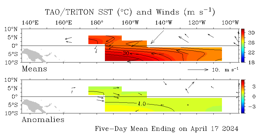
You can see below in the graphic which shows temperature along the Equator as a function of depth, both the magnitude of the anomalies and their size. You can now see where 2C (anomaly) water is impacting the area where the ONI is measured i.e. 170W to 120W. The 2C anomaly now extends to beyond 150W but not quite to 160W. The subsurface warm water appears to be making its way to the surface to some extent in the Eastern Pacific and also over at 160W which is probably related to the third Kelvin Wave. In the Central Pacific we now see a relatively small pod of warm water at about the Date Line where the westerly wind burst occurred and where we see above the beginning of one more Kelvin Wave. So far it seems to be fairly minor compared to what has occurred in prior months and has merged with the prior Kelvin Wave in terms of subsurface impacts. But that might change. It certainly has delayed the movement of the leading edge of the warmer water to 170W. At that point we are likely to see the ONI decline week to week. We may get some additional insight when we discuss the TAO/TRITON graphic.
The big issue is where will the +6C and +5C anomaly water go as it reaches the beaches of Ecuador? To the extent it surfaces, it can create convection and impact the Walker Circulation which could then provide positive feedback to this El Nino. But that warm water might tend to go north or south or both. That is part of the phase out process for an El Nino and that is where we are in the life of this El Nino. It is peaking and will soon begin its decline. But it is certainly taking its sweet time probably because of the large amount of the subsurface warm water. Water is a very good insulator: I believe it has the second highest specific heat capacity of all known substances. So that means that other than by mixing, that warm water under the surface will stay warm until it rises to the surface where it can be cooled by evaporation (while making clouds) or moves to the north where it will impact Mexico and the the Southern Coast of the U.S. That is part of the basis for models predicting that the ONI of this El Nino will continue to rise but I am a bit skeptical because I see it as rising to the east of the ONI measurement area and not being counted.
The bottom half of the graphic is not that useful in terms of tracking the progress of this Warm Event as it simply shows the thermocline between warm and cool water which pretty much looks like this as shown here during a Warm Event and you can see that the cooler water is not making it to the surface to the east along the coast of Ecuador. However, one is beginning to see the increase in the slope of the thermocline (look at the 25C dividing line for example which appears to have reached the surface). We can now begin to monitor the 20C Isotherm which is often thought of as being the middle or lower edge of the thermocline.where the slope is also steepening.
When I put all the information together I still conclude that I believe the ONI will soon peak and begin to decline. The possibility that there could be yet another Kelvin Wave forming, given the strength of the SOI, is a piece of information that at this point is difficult to assess. And there is the issue of how the Walker Circulation might extend the life of this Warm Event. The question of the Walker Circulation is not separate from the question of the forming of another Kelvin Wave. Pretty much all of the issues I am discussing are interrelated.
Back to the TAO/TRITON graphic below, notice that the 1.5C+ anomaly has reached 170W. When the leading edge of the warm water area moves beyond 170W, the anomalies in the western parts of Nino 3.4 are likely to start to decline. But at the same time, the subsurface warm water is coming to the surface and that makes the anomalies in the eastern part of Nino 3.4 larger. You can see there are two centers of warm surface water one related to the cumulative impact of the first two Kelvin Waves and the other at 170W representing the impact of the most recent third Kelvin Wave. Notice the 28C Isotherm. South of the Equator it extends over to beyond 140W but north of the Equator it does not extent very far north as there is even warmer water north of that isotherm. .
To me, this being a summer El Nino, the near-term potential impacts on CONUS may currently be over-hyped since the real impacts will be felt this Fall and Winter. But on the other hand, there are signs that this may develop into a very powerful El Nino in the Fall. So we have to watch what happens carefully..
For my own amusement, I calculate the ONI each week using a method that I have devised. To refine my calculation, I have divided the 170W to 120W ONI measuring area into five subregions (that I have designated A through E (from west to east) with a location bar shown under the TAO/TRITON Graphic) and have mentally integrated what I see below and recorded that in the table I have constructed. Then I take the average of the anomalies I estimated for each of the five subregions.
| ———————————————– | A | B | C | D | E | —————- |
So as of Monday August 10 in the afternoon working from the August 9 TAO/TRITON report, this is what I calculated which is basically the same as my calculation last week although the patterns of the anomalies have been changing around quite a bit but the changes have been cancelling each other out.
| Anomaly Segment | Estimated Anomaly |
| A. 170W to 160W | 1.4 |
| B. 160W to 150W | 1.2 |
| C. 150W to 140W | 1.5 |
| D. 140W to 130W | 2.0 |
| E. 130W to 120W | 2.2. |
| Total | 8.3 |
| Total divided by five subregions i.e. the ONI | (8.3)/5 = 1.7 |
My estimate of the Nino 3.4 ONI remains at 1.7. NOAA has today reported the weekly ONI as being 1.9 which is a significant increase from what was reported last week and much higher than my rough calculation. But it is important to remember that NOAA is reporting a weekly ONI and I am estimating a daily ONI. The increase in the NOAA estimated ONI is I beleive mostly due to the subsurface water in the Eastern Pacific backing up to the west as it comes to the surface. This warm water certainly impacts the weather in Ecuador and Peru but may not have a direct impact on weather in CONUS other than by spawning tropical cyclones which move north and enter the circulation of the Southwest Monsoon. That activity seems to have decreased recently.
Nino 4.0 is now reported as being 0.9. You can already see (in my calculation table) the gradient from West to East that has formed with the higher values in the East and the Western part of the Zone having a smaller anomaly which I believe has already begun to decline. But the new Kelvin Wave has arrived in the Nino 3.4 measurement area and will cause another rise in the ONI for the western part of the Nino 3.4 measurement area but so far that to me appears to me of smaller magnitude. This then may well result in a very complicated Walker Circulation pattern.
The real action is in Nino 1+2 which is reported as 2.6 which is down slightly from last week. The issue is how warm water off of Ecuador and Peru impacts CONUS weather. I think it has very little impact and that is what we are seeing right now.
Here is another way of looking at it:
.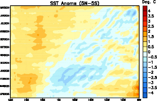
This Hovmoeller shows a lot of useful information which I have discussed in previous weeks and I will not repeat the same interpretation over and over again. Today I see a continuing tendency for the areas east of Nino 3.4 to be less warm than in prior weeks but continually expanding to the west which lead to higher ONI calculations. That could be an indication of this El Nino slowly working its way through the process of disposing of the subsurface very warm water. That is why we see the ONI values on a weekly basis increasing but it is the three-month average that eventually enters the official records.
Recent Impacts of Weather Mostly El Nino but possibly Also PDO and AMO Impacts.
I was not satisfied showing a 90 day and a 30 picture since the 30 day is subsumed into the 90 day so I decided to show three one-month pictures as I think that is a lot easier to follow. I do not plan to update the prior two months each week but monthly.
First the Temperature and Precipitation Departures from two months ago

Then the prior month’s 30-Day

And the current 30-Day which shows the more recent impacts

Re precipitaiton I think you can see the drying trend which is not exactly what you expect with an El Nino. For many parts of CONUS it is a cooling trend also which may be associated with an El Nino.
I wish NOAA would figure out how to produce graphics that work when you print them in black and white (hint crosshatching) as that would make it easier for those who like to print and read rather than squint at a screen for a long time. You can clealy see how the El Nino has dried up Mexico.
Pulling it All Together
We are in El Nino conditions now. The actually impacts on CONUS are not clear. We have had wetter conditions than usual in the Southwest but that has tappered off a bit. But this is the Summer so El Nino impacts on Summer conditions in the Northern Hemisphere are muted even though this is a powerful El Nino. So it is somewhat of a confusing situation as the impacts are not currently proportional to the current strength of this El Nino.
It is probably influencing the IOD to tend towards being positive thus providing a double whammy for parts of Asia and Australia. The length and intensity of this El Nino is still not clear mostly in terms of whether or not it will extend into the early part of 2016. All the computer models predict that it will last longer than my mental model suggests to me. The disagreement is in terms of a couple of months but a couple of months makes a difference in terms of agriculture and other economic impacts. Actually the JAMSTEC model is not very different from my assessment. We may or may not have a Pacific Climate Shift as the PDO+ may be simply related to the Warm Event (and quite frankly at this point appears to be). But for now we do have PDO+. The AMO being an overturning may be more predictable so the Neutral status moving towards AMO- is probably fairly reliable but not necessarily proceeding in a straight line. So none of this is very difficult to figure out actually if you are looking at say a five-year forecast.The research on Ocean Cycles is fairly conclusive and widely available to those who seek it out. I have provided a lot of information on this in prior weeks and all of that information is preserved in Part II of my report in the Section on Low Frequency Cycles 3. Low Frequency Cycles such as PDO, AMO, IOBD, EATS. It includes decade by decade predictions through 2050. Predicting a particular year is far harder. But we are beginning to speculate on the winter of 2016/201 which I believe will tend to be ENSO Neutral but I am not so sure that it will not lean towards being a cool event or at least closer to a La Nina than neutral. One thing is fairly certain for the U.S. it will be less wet and warmer than the winter of 2015/2016 which will be quite wet and cool. JAMSTEC is predicting that the Spring of 2017 will begin a mild La Nina.
TABLE OF CONTENTS FOR PART II OF THIS REPORT The links below may take you directly to the set of information that you have selected but in some Internet Browsers it may first take you to the top of Page II where there is a TABLE OF CONTENTS and take a few extra seconds to get you to the specific section selected. If you do not feel like waiting, you can click a second time within the TABLE OF CONTENTS to get to the specific part of the webpage that interests you.
A. Worldwide Weather: Current and Three-Month Outlooks: 15 Month Outlooks (Usefully bookmarked as it provides automatically updated current weather conditions and forecasts at all times. It does not replace local forecasts but does provide U.S. national and regional forecasts and, with less detail, international forecasts)
B. Factors Impacting the Outlook
1. Very High Frequency (short-term) Cycles PNA, AO,NAO (but the AO and NAO may also have a low frequency component.)
2. Medium Frequency Cycles such as ENSO and IOD
. Low Frequency Cycles such as PDO, AMO, IOBD, EATS.
C. Computer Models and Methodologies
D. Reserved for a Future Topic (Possibly Predictable Economic Impacts)
TABLE OF CONTENTS FOR PART III OF THIS REPORT – GLOBAL WARMING WHICH SOME CALL CLIMATE CHANGE. The links below may take you directly to the set of information that you have selected but in some Internet Browsers it may first take you to the top of Page III where there is a TABLE OF CONTENTS and take a few extra seconds to get you to the specific section selected. If you do not feel like waiting, you can click a second time within the TABLE OF CONTENTS to get to the specific part of the webpage that interests you.
D2. Climate Impacts of Global Warming
D3. Economic Impacts of Global Warming
D4. Reports from Around the World on Impacts of Global Warming.


