Written by Sig Silber
The recent extremes in the Continental U.S. weather: West versus East and North versus South have moderated. Spring is here and near-term projections now have high levels of uncertainty. The potential for an El Nino this coming winter is no clearer this Monday than it was last Monday.

This is the Regular Edition of my weekly Weather and Climate Update Report. Additional information can be found here on Page II of the Global Economic Intersection Weather and Climate Report.
On Saturday, the NOAA weekend unsupervised NOAA computers announced that NOAA had been incorrect in their revised April Outlook. On Sunday, the computer moderated their rebuke ever so slightly and today NOAA acceded to the perspective of the computers with the caveat that their 6 – 14 Day Outlooks have relatively low confidence. More on that later.
I have been asked why computer models are not perfect. Here are two good reasons:
A. The model is incomplete. This can occur for two reasons:
1. the people designing the model are unaware of all the factors influencing the outcome so one or more factors are not included in the model.
2. the people designing the model are aware of other factors but either the data to properly include them is unavailable or the cost to collect the data is deemed to be larger than the benefit or the funding is simply unavailable. The Earth is a large Planet and the atmosphere and oceans have three dimensions. So depending on the desired degree of resolution, that is a lot of data. The following from the History of Numerical Weather Forecast is a pretty good introduction to weather forecasting models:
Until the end of the 19th century, weather prediction was entirely subjective and based on empirical rules, with only limited understanding of the physical mechanisms behind weather processes. In 1901 Cleveland Abbe, founder of the United States Weather Bureau, proposed that the atmosphere is governed by the same principles of thermodynamics and hydrodynamics that were studied in the previous century. In 1904, Vilhelm Bjerknes derived a two-step procedure for model-based weather forecasting. First, a diagnostic step is used to process data to generate initial conditions, which are then advanced in time by a prognostic step that solves the initial value problem. He also identified seven variables that defined the state of the atmosphere at a given point: pressure, temperature, density, humidity, and the three components of the flow velocity vector. Bjerknes pointed out that equations based on mass continuity, conservation of momentum, the first and second laws of thermodynamics, and the ideal gas law could be used to estimate the state of the atmosphere in the future through numerical methods. With the exception of the second law of thermodynamics, these equations form the basis of the primitive equations used in present-day weather models.
This article also might be of interest in terms of background on the history of the development of weather forecasting models.
Of course there has been much progress since then but you get the idea that one has to be able to describe the current conditions of the atmosphere (and land and ocean surfaces) to be able to make forecasts.
One approach to deal with lack of data is to extrapolate missing data using equations that estimate the missing data based on the actual observations. That provides a way to initialize a model. An improvement on that is to vary the estimates of the initial conditions (consistent with the distribution of variations in the real world and there is the rub) and run the models to see how sensitive the models are to small changes in the estimates of the initial conditions. This is one version of “ensembles” a fancy word for a collection of related things. You can have an ensemble of different initial conditional assumptions or an ensemble of slightly different models and the “spread” of the solutions is assumed to be a measure of the confidence one should have in the forecasts. I leave it to the reader to decide if that approach is consistent with how they arrive at confidence about the future. I am not saying that there is a better approach, but I am saying that if the model is wrong and “sensitivity” analysis indicates that small changes in assumptions or internal formulae for parametrization do not cast doubt on the forecast, that forecast will still be less than useful if the model itself is incomplete or just plain wrong.
Sufficient computational capacity is also important. Here is a blog post on that topic, which is a little out of date, but purports to describe the situation in the U.S. It is possible that some of the issues discussed in that blog post have been addressed since it was written, but my experience is that other nations lead the U.S. If you do not like the situation, talk to Congress. NOAA needs to be reorganized, streamlined, given new leadership and then provided adequate funding. Part of the situation is a result of the decision to provide opportunities for the private sector and not have the Federal solution so comprehensive that there was no room for the private sector to add value. It is a delicate balancing act.
B. The model is based on historical data but the situation has changed.
Thus the model continues to interpret the inputs as they should be interpreted consistent with the situation at the time the data was collected. Hence my conclusion that computer models essentially “predict the past not the future” which could be reworded to be less inflammatory as models “predict the future in the same way they would have predicted a similar situation in the past and thus their prediction of the future is essentially the same as predicting the past”.
The reason for the above is that the way you build a model is by collecting information on the results that have occurred in the past when certain conditions applied. A real good example would be cyclones where we have theoretical and observed data on how tropical waves evolve into cyclones. But what if many of the factors in the lifecycle of cyclones change over time due to Climate Change. Will our models still be as effective as in the past?
From a mathematician’s perspective, a relationship is valid only if the domain of samples used in the creation of the model includes the values used in the running of the model. From a practical perspective, you have no way to calibrate and test such a model if you have no data for situations faced that have never been faced before. We run into this problem with Climate Change models. The domain of data does not include carbon dioxide concentrations of 400 PPM or average temperatures greater than what we had for the last thirty years.
So the models are informed guesses as to how things might be in the future. The model designers attempt to calibrate their models against historical data but we do not have historical data where carbon dioxide levels are as high as today nor average temperatures including ocean temperatures are as high as today. Efforts to use paleo data are actually quite laughable since you normally do not improve an accuracy problem by deciding to use a more approximate set of data.
SUMMARY
For weather forecasting models, the incompleteness is the bigger problem. For Climate Change models, their use beyond the envelop of where the results are able to be calibrated is the larger problem.
Before getting into the current situation I realize I forgot to post this update last week. Actually I am not sure when Queensland (no that is not where the U.S. Open Tennis Tournament is held) updated their precipitation forecast.
Worldwide Precipitation Outlook
The Australian Queensland Bureau of Meteorology uses the SOI to make a worldwide precipitation forecast and here it is. It is interesting because it is based on just one variable: the air pressure differential between Tahiti and Darwin Australia.

You can read about it here. I have not researched the skill level of this tool and the SOI is mostly a tropical index, but I include it because it is interesting.
I have not checked it out on a worldwide basis but it seems to have done a very good job of projecting U.S. precipitation so far this Spring. It is pretty amazing given that it is based on just one variable the SOI, the variable that NOAA seems to ignore. The SOI has been in neutral territory all winter i.e. the 2014/2015 winter but NOAA has chosen to ignore that reality. That is one reason why their seasonal forecasts this winter have been so screwy.
I thought I would repeat this animation. IT TAKES A FEW SECONDS TO RUN SO PLEASE BE PATIENT. It shows the Warm Event along the Equator dissipating or turning into a Modoki Type II i.e. cold Eastern Pacific, warm Central Pacific (mostly west of the Date Line) and warm water off the Northwest Coast of the U.S. But is the story changing? Is the Modoki cleaning up its act and going Traditional? Watch the last several frames carefully! The Gulf of Mexico has changed also. The warming in the Gulf of Mexico may have greater short-term significance on CONUS weather.
Progress of the Warm Event
I thought I would recalculate the ONI again as I have been doing recently. The little tick marks on the chart can be used instead of a ruler. When I print out this graphic one tick is about one centimeter. So you can use a ruler or just estimate the number (including fractions) of tick marks.
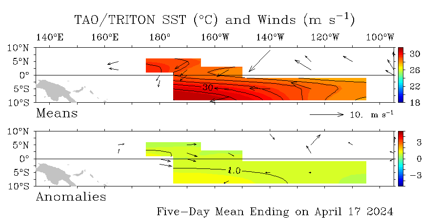
First I want to call your attention to the fact that we now have surface temperature and wind anomalies in the Eastern Pacific. The arrows east of 120W now point North. That does not mean we have Southerly winds (see the upper graphic which shows the actual values not the anomalies) but that the Easterlies have relaxed and now have a southerly vector in them. We certainly have more warmish water off of Ecuador and that is recent and makes the pattern a little more like a Traditional El Nino. It is kind of a bimodal distribution of temperature anomalies. To me it seems unusual. We will see how it continues to evolve. Remember that 28C is what makes the weather get interesting.
Also remember there is a lag between ocean conditions and weather impacts on land. People tend to forget that it takes time for ocean conditions to propagate over land. Weather is not digital; it is analog.
So as of Monday April 6 in the afternoon working from the April 5 TAO/TRITON report, this is what I observed.
| Anomaly Segment | Midpoint | Length on Equator in number of five degrees of latitude (ticks) | Midpoint X Length (tempxticks) |
| -0.5C to 0C | -0.25 | 0 | 0 |
| 0C to +0.5C | +0.25 | 0 | 0 |
| +0.5C to 1.0C | +0.75 | 4 | 3.0 |
| 1.0C to 1.5C | +1.25 | 1 | 1.25 |
| Total | 5 Ticks (or 5 centimeters) | 4.25 /5= 0.85 C Estimated ONI |
My estimate of the Nino 3.4 ONI is now 0.85 which is a respectable value. Notice it is now warm both north of the Equator and south of the Equator which is a big change. This symmetry around the Equator has however decreased a bit and this decreases the accuracy of my estimation approach. I think the NOAA reading is too low but remember that NOAA is providing a weekly average and I am estimating a daily value. So if the ONI is rising or falling dramatically, the average will lag a daily reading but that is not the case right now. The NOAA estimate is impacted to a slight extent by some cooler water as you can see above but I do not think that is a major factor.
The real story here however still remains Nino 4.0 where the ONI there is now reported by NOAA to be 1.1. Nino 3.4 ONI is officially reported by NOAA as 0.7 but probably is a bit higher as I have calculated above. Nino 1 and 2 are in play. Oh my gosh! 1.4! Something is clearly happening in the Equatorial Pacific. It started as a Traditional El Nino, changed to a Modoki-ish event that did not begin in the way that a Modoki usually begins, and now appears to be morphing into more of a Traditional El Nino. But in my opinion the pattern still most closely resembles a Modoki Type II. That might change.
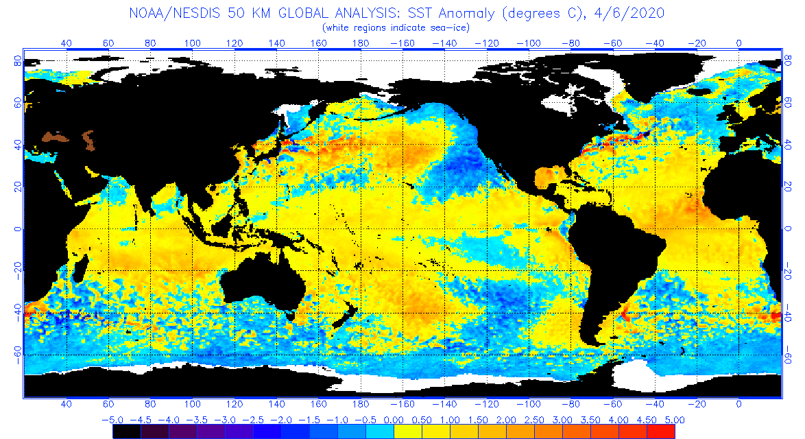
Now this week’s weekly SST Departures.

This is similar to last week which was a big change from the prior week.
This animation may provide some additional insight. This graphic shows the absolute temperatures not the anomalies. You can see the tendency for warm water to pool in the Western Pacific which in the extreme is La Nina Conditions. When it returns to the East you get what is called an El Nino. If the warm water is mostly near the Date Line, it is a Modoki.
Notice the action north and south of the Equator.
Here is a total Pacific view which to me shows it is still a Modoki Type II. Unlike the above graphic which shows the absolute temperatures, this shows the anomalies compared to average conditions. Notice the diagonal pattern of warm temperatures which is suggestive of a Modoki Type II plus the westward extension of the warmest anomalies.
It is an active pattern that is for sure. Both animations show weekly averages. So the last frame may be current or not depending on when you view the animation.
From Japan. I have not posted this before mostly because I did not notice it until Sunday. It is a bit old in the sense of having been run on February data. I do not know how frequently this graphic updated. But to me it shows a Modoki Type II pattern which looks a lot like simply a Modoki with a positive PDO.

And here is their precipitation forecast.

It is very different from the Queensland forecast and similar to the earlier NOAA forecast and for the U.S., coincides with today’s NOAA Outlook.
I wish I had noticed it sooner.
Short-term Outlook –
Let us take a look at what was issued today April 6, 2015. It will auto-update every day so it will be changing day by day (and thus be up to date whenever you elect to read this report) but my comments as well as the comments of NOAA may become out of sync with the map since these comments do not auto-update.
Generally I only show the “second week” namely the 8 -14 Day Outlook. The first week (6 – 10 Day Outlook) together with much additional information on current weather patterns and near-term forecasts can be found in Part II of my report, but 8 – 14 days covers most of the 6 – 14 day period. However, that is not true today for the Temperature Outlook which changes dramatically in the middle of the 6 – 14 Day period.
Here is the updated April Temperature Outlook issued on March 31, 2015

And here is the April 8 – 14 Day Temperature Outlook issued today April 6, 2015.

Here is the updated Precipitation Outlook for April issued on March 31, 2015

Here is the 8 – 14 Day Precipitation Outlook issued today April 6, 2015.

I guess you can see how the colder and wetter than climatology Southwest has been reintroduced after being removed with the March 31 Update. Remember that the 6 – 14 day outlook only covers 9 days not the full month.
And here are excerpts from the NOAA release today April 6, 2015.
“6-10 DAY OUTLOOK FOR APR 12 – 16 2015
TODAY’S MODELS EXHIBIT FAIR TO GOOD AGREEMENT ON THE 500-HPA HEIGHT PATTERN OVER NORTH AMERICA. MOST MODEL SOLUTIONS DEPICT A RIDGE OVER THE EASTERN PACIFIC AND ABOVE NORMAL HEIGHTS EXTENDING FROM THE WESTERN ATLANTIC TO THE EASTERN CONUS. GENERALLY BELOW NORMAL HEIGHTS ARE INDICATED OVER THE SOUTHWEST AND ALASKA. THE LARGEST DIFFERENCES ARE OVER THE CENTRAL PORTIONS OF THE CONUS, WHERE THE 500-HPA HEIGHTS FROM THE 6Z DETERMINISTIC GFS ARE LOWER THAN THE 0Z EUROPEAN AND CANADIAN ENSEMBLE MEANS. THE 0Z CANADIAN ENSEMBLE MEAN HAS THE HIGHEST HEIGHTS OVER THE NORTH-CENTRAL CONUS.
TODAY’S 0Z AND YESTERDAY’S 12Z CANADIAN ENSEMBLE MEANS MAKE UP 40 PERCENT OF THE 500-HPA MANUAL BLEND, WHICH SLIGHTLY FAVORS THE EUROPEAN AND CANADIAN SOLUTIONS OVER THE GFS BASED SOLUTIONS. THE 6Z GFS ENSEMBLE MEAN AND GFS SUPERENSEMBLE ARE INCLUDED IN THE MANUAL BLEND AS THOSE TWO MODELS HAVE RECENT SKILL ON PAR WITH THE EUROPEAN AND CANADIAN, WHILE THE ANALOG CORRELATION FROM THE GFS SUPERENSEMBLE IS THE SECOND HIGHEST OF THE AVAILABLE MODELS.
THE SURFACE TEMPERATURE OUTLOOK SHOWS MOSTLY ABOVE NORMAL TEMPERATURES OVER MOST OF THE CONUS, REFLECTING THE NEAR TO ABOVE NORMAL HEIGHTS OVER THE ENTIRE CONUS. THE TROUGH OVER THE SOUTHWEST IS NOT CHARACTERIZED BY LARGE MAGNITUDE ANOMALIES AT 500-HPA, SO AN AREA OF NEAR NORMAL TEMPERATURES IS INDICATED THERE. UPPER-LEVEL VARIABILITY INDICATES SOME TRANSIENT TROUGH ACTIVITY AND SLIGHTLY BELOW NORMAL HEIGHTS OVER THE NORTHERN ROCKIES RESULTED IN A FORECAST OF NEAR NORMAL TEMPERATURES FOR THAT REGION. MODERATE STRENGTH TROUGHING OVER FORECAST OVER MUCH OF ALASKA ALLOWS FOR SOME COLDER AIR TO SETTLE OVER THE STATE, RESULTING IN A FORECAST OF BELOW NORMAL TEMPERATURES, WITH THE HIGHEST PROBABILITIES NEAR THE WEST COAST.
BELOW MEDIAN PRECIPITATION IS FORECAST FROM THE PACIFIC NORTHWEST TO THE NORTHERN HIGH PLAINS DUE TO UPSTREAM RIDGING. THE PROBABILITIES ARE LOW TO ACCOUNT FOR THE UNCERTAINTY DUE TO TRANSIENT TROUGHS POTENTIALLY COMING SLIGHTLY FURTHER SOUTH THAN MOST MODELS CURRENTLY DEPICT. A LARGE AREA OF ABOVE MEDIAN PRECIPITATION IS FORECAST FROM THE SOUTHWEST TO THE SOUTHEAST AND NORTHWARD TO THE GREAT LAKES. THAT AREA REFLECTS THE TROUGHING OVER THE SOUTHWEST AND THE STRONG SOUTHERLY FLOW AROUND THE SURFACE HIGH PRESSURE EXTENDING OVER THE EASTERN CONUS FROM THE ATLANTIC. LOW PRESSURE OVER THE GULF OF ALASKA FAVORS ABOVE MEDIAN PRECIPITATION FOR SOUTHEAST ALASKA, WHILE NORTHERLY FLOW FAVORS BELOW MEDIAN PRECIPITATION FOR NORTHWEST ALASKA.
FORECAST CONFIDENCE FOR THE 6-10 DAY PERIOD: BELOW AVERAGE, 2 OUT OF 5, DUE TO DISAGREEMENT AMONG MODELS ON THE AMPLITUDE OF TROUGHING OVER THE NORTHERN GREAT PLAINS AND DISAGREEMENT AMONG THE SURFACE PARAMETER TOOLS.
8-14 DAY OUTLOOK FOR APR 14 – 20 2015
MODEL SOLUTIONS DURING THE 8-14 DAY PERIOD SEEM TO BE IN TWO DISTINCT FLOW REGIMES, ONE DEPICTED BY THE GFS BASED SOLUTIONS AND ONE CAPTURED BY THE EUROPEAN AND CANADIAN ENSEMBLE MEAN SOLUTIONS. THE MODELS AGREE UPON A RIDGE NEAR THE PACIFIC NORTHWEST, TROUGHING OVER THE SOUTHWEST, AND A RIDGE EXTENDING OVER THE SOUTHEAST FROM THE ATLANTIC. THE MODELS DISAGREE ON TROUGHING OVER THE NORTHEAST, THE EASTWARD EXTENT OF THE RIDGING OVER THE PACIFIC NORTHWEST, AND THE HEIGHTS OVER ALASKA. THE 0Z AND YESTERDAY’S 12Z GEFS MEAN SOLUTIONS EXHIBIT LARGE DISAGREEMENTS OVER THE NORTHERN GREAT PLAINS AND GREAT LAKES WITH THE AVAILABLE EUROPEAN AND CANADIAN ENSEMBLE MEANS FROM THE SAME INITIALIZATION TIMES. SUBJECTIVELY ASSESSED SPREAD AMONG THE MODEL SOLUTIONS IS HIGHER THAN IN MANY CASES DURING THE PAST 30 DAYS. ALSO, THE GEFS SOLUTIONS EXHIBIT VERY LITTLE CONSISTENCY FROM RUN TO RUN.
THE EUROPEAN AND CANADIAN SOLUTIONS WERE PREFERRED IN THE 500-HPA MANUAL BLEND DUE TO THE RUN-TO-RUN CONSISTENCY ISSUES. TODAY’S 0Z AND YESTERDAY’S 12Z CANADIAN ENSEMBLE MEAN WERE GIVEN EQUAL WEIGHTING AND COMPRISE 50 PERCENT OF THE 500-HPA MANUAL BLEND. THOSE MODELS HAVE ANOMALY CORRELATION SCORES ON PAR WITH THE EUROPEAN ENSEMBLE MEAN DURING THE PAST 60 DAYS AND HAVE THE HIGHEST ANALOG CORRELATION SCORES.
ABOVE NORMAL TEMPERATURES ARE FAVORED ACROSS THE WESTERN CONUS, ASSOCIATED WITH THE ABOVE NORMAL HEIGHTS. RIDGING FROM THE WESTERN ATLANTIC FAVORS ABOVE NORMAL TEMPERATURES OVER THE SOUTHEAST. TROUGHING OVER THE SOUTHWEST SUPPORTS BELOW NORMAL TEMPERATURES FOR THE SOUTHERN GREAT PLAINS AND NEW MEXICO, WHILE TROUGHING EXTENDING SOUTHWARD FROM CANADA SUPPORTS BELOW NORMAL TEMPERATURES OVER THE GREAT LAKES. ABOVE NORMAL TEMPERATURES ARE FAVORED OVER SOUTHERN ALASKA DUE TO SOUTHERLY ANOMALOUS FLOW AS THE UPPER-LEVEL TROUGH IS FORECAST TO WEAKEN DURING THIS PERIOD, AS COMPARED TO THE 6-10 DAY PERIOD.
A TENDENCY TOWARD SPLIT FLOW OVER THE WESTERN CONUS AND RIDGING OVER THE PACIFIC NORTHWEST FAVOR BELOW MEDIAN PRECIPITATION FROM THE PACIFIC NORTHWEST TO THE NORTHERN GREAT PLAINS, ALTHOUGH PROBABILITIES ARE LOW EAST OF THE ROCKIES TO REFLECT UNCERTAINTY ON THE IMPACT OF TROUGHS MOVING OVER THE TOP OF THE RIDGE. SOUTHERN STREAM TROUGHING AND SOUTHERLY FLOW AT LOW LEVELS FAVOR ABOVE MEDIAN PRECIPITATION FROM THE SOUTHWEST TO THE SOUTHEAST AND NORTHWARD TO THE NORTHEAST. MEAN LOW PRESSURE OVER THE GULF OF ALASKA FAVORS ABOVE MEDIAN PRECIPITATION FOR SOUTHERN ALASKA AND BELOW MEDIAN PRECIPITATION FOR THE NORTHERN THIRD OF THE STATE.
FORECAST CONFIDENCE FOR THE 8-14 DAY PERIOD IS: BELOW AVERAGE, 2 OUT OF 5, DUE TO DIFFICULTIES IN THE PREDICTION OF A SPLIT-FLOW OVER THE CONUS.“
Analogs to Current Conditions
Now let us take a detailed look at the “Analogs” which NOAA provides related to the 5 day period centered on 3 days ago and the 7 day period centered on 4 days ago. “Analog” means that the weather pattern then resembles the recent weather pattern and was used in some way to predict the 6 – 14 day Outlook.
Here are today’s analogs in chronological order although this information is also available with the analog dates listed by the level of correlation. I find the chronological order easier for me to work with. There is a second set of analogs associated with the outlook but I have not been analyzing this second set of information. This first set applies to the 5 and 7 day observed pattern prior to today. The second set which I am not using relates to the forecast outlook 6 – 10 days out to similar patterns that have occurred in the past during the dates covered by the 6 – 10 Day Outlook. That may also be useful information but they put this set of analogs in the discussion with the other set available by a link so I am assuming that this set of analogs is the most meaningful.
Analog Centered Day | ENSO Phase | PDO | AMO | Other Comments |
| 1954 April 1 | La Nina | – | + | Right after an El Nino |
| 1967 March 16 | Neutral | – | – | |
| 1969 March 30 | El Nino | – | – | |
| 1982 April 3 | El Nino | + | – | Start of powerful traditional El Nino |
| 1982 April 4 | El Nino | + | – | Start of powerful traditional El Nino |
| 2003 April 1 | Neutral | + | + | Right after an El Nino Modoki Type I |
| 2003 April 3 | Neutral | + | + | Right after an El Nino Modoki Type I |
| 2008 March 27 | Neutral | – | + |
This week there are four ENSO Neutral and one La Nina and three El Nino analogs. So that is a big change from last week. NOAA provides me with ten but I discard the duplicates. The 1982 April 3 and 4 analogs are very interesting as that was a late arriving but very powerful traditional El Nino. It could tell us something about this coming winter. Of interest that particular El Nino was not associated with a Pacific Climate Shift. The Ocean Phases of the analogs this week are inconclusive as all four of the McCabe et al conditions are represented. The spread of dates of the analogs exceed a month which indicates the complexity of the onset of Spring this year.

Red is a high likelihood of drought, blue the opposite.
Back to the Current Situation:
Sometimes it is useful to take a look at the location of the Jet Stream or Jet Streams.

And sometimes the forecast is revealing. Below is the forecast out five days. I do not see the split Jet Stream in this forecast so presumably it occurs later in the period. But you do see how there could be a trough in the center of CONUS if the middle and lower layers of the atmosphere are significantly influenced by the Jet Stream.

To see it in animation, click here.
This longer animation shows how the jet stream is crossing the Pacific and when it reaches the U.S. West Coast is going every which way. One can imagine that attempting to forecast this 6 – 14 days out is quite challenging and NOAA is having fits attempting to guess how this will play out over a 14 day period especially for the Southwest.
And below is another view which highlights the surface highs and the lows re air pressure on Day 3. The RRR is gone presumably for the Spring and Summer and may not be a factor this coming winter if there is a traditional El Nino.

And here is Day 6. There is not much to see which suggests that Winter is no longer a factor and weather will be more local except perhaps where the North American Monsoon is a factor a few months out.

More El Niño Discussion
The view of El Nino as a 2014/2015 event appears to be morphing into a view that it is a 2015/2016 event. But all predictions about El Nino for next winter must be tempered by what is called the Spring Prediction Barrier (SPB). Nevertheless, an El Nino this coming winter is a real possibility.
It is useful to understand where ENSO is measured.

Of most interest to NOAA is 120 W to 170 W labeled Nino 3.4 as that is where the ONI Index most often used in the U.S. for defining ENSO Events is measured. More information can be found here. In Asia they tend to pay more attention to Nino 3
And now the low-level wind anomalies.

This is a lot of change since last week. I believe the above graphic is current as of April 3 but today is April 6 so that leaves a bit to be desired given the last few days of the SOI. Notice the significant amount of area that last week was in shades of brown but now is blue. The big westerly wind burst of more than a month ago is history but is still having its impacts but it has not been reinforced and in fact this week was reversed.
The Southern Oscillation Index (SOI) this week has been strictly in La Nina territory. Today’s reading of +8.3 is a La Nina reading. The SOI fluctuates based on local weather conditions in Tahiti and Darwin Australia which is why the 30 and 90 day averages are more significant than the daily values. The 30 day average of -10.3 is certainly consistent with El Nino conditions (a 30 day average of -8.0 or more negative (using the standard SOI Index) is considered to be consistent with El Nino conditions). The 90 day average is currently -6.4 which is not sufficiently negative to be considered consistent with El Nino conditions. You can always find the updated daily values and the 30 and 90 day averages here.
31 March 2015 -8.8
1 April 2015 +4.7
2 April 2015 +13.4
3 April 2015 +1.8
4 April 2015 +0.3
5 April 2015 +7.7
6 April 2015 +8.3
The Kelvin Wave graphic is very interesting this week. It is really the Upper Ocean Heat Anomaly.

This is interesting. The Kelvin wave which appeared to be stalled two weeks ago last week was clearly progressing eastward. Remember the bottom of the graphic is the current readings and as you look up you see basically day by day the historical progression of these waves. When the pattern started to deviate from 45 degrees and became more vertical two weeks ago, to me that signified a decreasing impact of the Kelvin Wave. But that changed last week but the playing out may be showing up again but not as pronounced. Of course the Kelvin Wave may be making landfall now.
We need to switch our attention to the western side of the wave and there it does appear that we see a potential upwelling phase beginning in the far western Pacific that intense blue patch plus some sign of the impacts of the downwelling phase slightly diminishing along the Equator. This Kelvin wave has been far more intense than I thought it would be and we see this reflected in the Nino readings. Credit the SOI up until this past week. An upwelling Kelvin Wave could signal the end of this Warm Event or just a break in the action.
Since we looked at the Upper Ocean Anomalies let’s also look at the Surface Anomalies.

You can see the change from last week but it is not dramatic but confirms the warm water in the Eastern Pacific. It still looks like mostly a Central Pacific or Date Line Warm Event not a Traditional/Canonical El Nino. But it clearly is different this past two weeks and the interpretation is now up for grabs. .
And finally the latest model results released by NOAA oddly on April 4, 2015 not today.

There are two ways to look at this graphic assuming the projections are correct. One way is that we are in an El Nino that started in Aug-Sept-Oct of 2014 and may continue through the summer and possibly into next winter. Another way is that we had a near or marginal El Nino Modoki Type II starting in Aug-Sept-Oct 2014 which has just ended and we may be starting a Traditional El Nino Event. I think the latter is a more useful approach. I say that because the weather this past winter was consistent with there not having been a Traditional El Nino Event this past winter. What the future holds remains to be seen.
The continued tendency for models to show a strengthening of this El Nino is reasonable (given the Positive nature of the PDO right now) but questionable given the reality of what is called the Spring Prediction Barrier (SPB). If I was preparing that graphic, I would definitely have a footnote on the SPB to avoid misleading the reader. The upper left mini-graphic which is hard to see in this larger graphic without using the zoom feature available in most brousers, forecasts a Traditional El Nino conditions for April – May – June. We will see.
I thought I would include the below that I never used before. It shows that on a Nino 3.4 basis this now qualifies as an El Nino (it did not until the end of March). There are other criteria than just the Nino 3.4 to make the call. But looking below you see the requisite five three-month averages of 0.5 or greater. However two of the five are just 0.5 so if this were the end of this Warm Event, it would probably be the weakest El Nino ever called.

Pulling it All Together.
There has been a short-term strengthening of this Warm Event at the wrong time of the year. It is looking a bit more like a Traditional El Nino. NOAA expresses a point of view that I can neither confirm nor contradict (I have not done the research to do either) that if this Warm Event extends through the summer, the odds of an El Nino next winter are very good. It does not seem unreasonable to me but I do not have the data to assess it. For the Spring and Fall it should have minimal impact. Because right now we still have more of a Modoki-ish pattern than a Traditional Pattern, I have guarded confidence in the NOAA Three-Month precipitation Outlook. I also have no confidence in the longer-term outlook and neither does NOAA because it depends so much on whether or not this winter is an El Nino Winter and it is too soon to tell.
The PDO is showing very high readings which could signify the beginning of a climate shift in the Pacific which would be very significant for World weather for two or three decades. It will take three years before we know if that has occurred. At this point I am not at all convinced that this is the time that the flipping will occur but it might or it might take a strong La Nina to signal that change. I am inclined to think the latter so I am thinking that will occur in four or five years, but we will see. I am highly confident that the PDO will become consistently positive either now or within five years. I am starting to prepare a report on the economic impacts and investment opportunities that might follow such a Climate Shift.
Click Here for the Econointersect Weather and Climate Page II where you will find:
- A more complete set of NOAA and other agency graphics (including international agencies) that auto update. So this includes both short term- and seasonal “updates”. Most of the graphics will ALWAYS be up to date even if my commentary on the graphics is not. I update my commentary when it seems necessary and certainly every Monday, but some of these graphics auto update every six hours.
- Economic and other Impacts of major weather events. Not sure there is any other place to obtain this information consistently other than very specialized subscription services.
- Information on Climate Cycles both those which are fairly short term i.e. less than a decade in duration and multi-decadal cycles.
- Economic and other Impacts of those Climate Cycles which are referred to by the IPCC as Internal Variability as opposed to secular Climate Change which is always in the same direction. Again I am not sure if there is another source for this information where it is pulled together in one place as I have.
Click Here for Page III which deals with Global Warming.
- Information on Anthropogenic Global Warming science i.e. the secular change in our climate that overlays both short-term weather and historical climate cycles as well as black swan events like volcanic eruptions. I prefer to call this Global Warming as it is the warming that triggers the other changes.
- Economic and other Impacts of Global Warming. The IPCC AR5 WG2 attempts to describe and quantify these and I have some excerpts from their report. Over time I will go beyond their report as it is very deficient.


